Fisher's exact test

Last updated

Fisher's exact test is a statistical significance test used in the analysis of contingency tables. [1] [2] [3] Although in practice it is employed when sample sizes are small, it is valid for all sample sizes. It is named after its inventor, Ronald Fisher, and is one of a class of exact tests, so called because the significance of the deviation from a null hypothesis (e.g., p-value) can be calculated exactly, rather than relying on an approximation that becomes exact in the limit as the sample size grows to infinity, as with many statistical tests.

Contents

Fisher is said to have devised the test following a comment from Muriel Bristol, who claimed to be able to detect whether the tea or the milk was added first to her cup. He tested her claim in the "lady tasting tea" experiment. [4]

Purpose and scope

A teapot, a creamer and teacup full of tea with milk--can a taster tell if the milk went in first? Nice Cup of Tea.jpg
A teapot, a creamer and teacup full of tea with milk—can a taster tell if the milk went in first?

The test is useful for categorical data that result from classifying objects in two different ways; it is used to examine the significance of the association (contingency) between the two kinds of classification. So in Fisher's original example, one criterion of classification could be whether milk or tea was put in the cup first; the other could be whether Bristol thinks that the milk or tea was put in first. We want to know whether these two classifications are associated—that is, whether Bristol really can tell whether milk or tea was poured in first. Most uses of the Fisher test involve, like this example, a 2 × 2 contingency table (discussed below). The p-value from the test is computed as if the margins of the table are fixed, i.e. as if, in the tea-tasting example, Bristol knows the number of cups with each treatment (milk or tea first) and will therefore provide guesses with the correct number in each category. As pointed out by Fisher, this leads under a null hypothesis of independence to a hypergeometric distribution of the numbers in the cells of the table.

With large samples, a chi-squared test (or better yet, a G-test) can be used in this situation. However, the significance value it provides is only an approximation, because the sampling distribution of the test statistic that is calculated is only approximately equal to the theoretical chi-squared distribution. The approximation is poor when sample sizes are small, or the data are very unequally distributed among the cells of the table, resulting in the cell counts predicted on the null hypothesis (the "expected values") being low. The usual rule for deciding whether the chi-squared approximation is good enough is that the chi-squared test is not suitable when the expected values in any of the cells of a contingency table are below 5, or below 10 when there is only one degree of freedom (this rule is now known to be overly conservative [5] ). In fact, for small, sparse, or unbalanced data, the exact and asymptotic p-values can be quite different and may lead to opposite conclusions concerning the hypothesis of interest. [6] [7] In contrast the Fisher exact test is, as its name states, exact as long as the experimental procedure keeps the row and column totals fixed, and it can therefore be used regardless of the sample characteristics. It becomes difficult to calculate with large samples or well-balanced tables, but fortunately these are exactly the conditions where the chi-squared test is appropriate.

For hand calculations, the test is feasible only in the case of a 2 × 2 contingency table. However the principle of the test can be extended to the general case of an m × n table, [8] [9] and some statistical packages provide a calculation (sometimes using a Monte Carlo method to obtain an approximation) for the more general case. [10]

The test can also be used to quantify the overlap between two sets. For example, in enrichment analyses in statistical genetics one set of genes may be annotated for a given phenotype and the user may be interested in testing the overlap of their own set with those. In this case a 2 × 2 contingency table may be generated and Fisher's exact test applied through identifying

  1. Genes that are provided in both lists
  2. Genes that are provided in the first list and not the second
  3. Genes that are provided in the second list and not the first
  4. Genes that are not provided in either list

The test assumes genes in either list are taken from a broader set of genes (e.g. all remaining genes). A p-value may then be calculated, summarizing the significance of the overlap between the two lists. [11]

Derivation

[12]

   Class I     Class II  Row Total
Blueaba + b
  Red  cdc + d
Column Totala + cb + da + b + c + d (=n)


Derivation

We set up the following probability model underlying Fisher’s exact test.

Suppose we have blue balls, and red balls. We throw them together into a black box, shake well, then remove them one by one until we have pulled out exactly balls. We call these balls “class I” and the remaining balls “class II”.

The question is to calculate the probability that exactly blue balls are in class I. Every other entry in the table is fixed once we fill in one entry of the table.

Suppose we pretend that every ball is labelled, and before we start pulling out the balls, we permutate them uniformly randomly, then pull out the first balls. This gives us possibilities.

Of these possibilities, we condition on the case where the first balls contain exactly blue balls. To count these possibilities, we do the following: first select uniformly at random a subset of size among the class-I balls with possibilities, then select uniformly at random a subset of size among the class-II balls with possibilities.

The two selected sets would be filled with blue balls. The rest would be filled with red balls.

Once we have selected the sets, we can populate them with an arbitrary ordering of the blue balls. This gives us possibilities. Same for the red balls, with possibilities.

In full, we have
possibilities. Thus the probability of this event is

Another derivation:

Derivation

Suppose each blue ball and red ball has an equal and independent probability of being in class I, and of being in class II. Then the number of class-I blue balls is binomially distributed. The probability there are exactly of them is , and the probability there are exactly of red class I balls is .

The probability that there are precisely of class I balls, regardless of number of red or blue balls in it, is .

Thus, conditional on having class I balls, the conditional probability of having a table as shown is

Example

For example, a sample of teenagers might be divided into male and female on one hand and those who are and are not currently studying for a statistics exam on the other. For example, we hypothesize that the proportion of studying students is higher among the women than among the men, and we want to test whether any difference in proportions that we observe is significant.

The data might look like this:

   Men     Women  Row total
Studying1910
  Not-studying  11314
Column total121224

The question we ask about these data is: Knowing that 10 of these 24 teenagers are studying and that 12 of the 24 are female, and assuming the null hypothesis that men and women are equally likely to study, what is the probability that these 10 teenagers who are studying would be so unevenly distributed between the women and the men? If we were to choose 10 of the teenagers at random, what is the probability that 9 or more of them would be among the 12 women and only 1 or fewer from among the 12 men?

First example

Before we proceed with the Fisher test, we first introduce some notations. We represent the cells by the letters a, b, c and d, call the totals across rows and columns marginal totals, and represent the grand total by n. So the table now looks like this:

   Men     Women  Row Total
Studyingaba + b
  Non-studying  cdc + d
Column Totala + cb + da + b + c + d (=n)

Fisher showed that conditional on the margins of the table, a is distributed as a hypergeometric distribution with a+c draws from a population with a+b successes and c+d failures. The probability of obtaining such set of values is given by:

where is the binomial coefficient and the symbol ! indicates the factorial operator. This can be seen as follows. If the marginal totals (i.e. , , , and ) are known, only a single degree of freedom is left: the value e.g. of suffices to deduce the other values. Now, is the probability that elements are positive in a random selection (without replacement) of elements from a larger set containing elements in total out of which are positive, which is precisely the definition of the hypergeometric distribution.

With the data above (using the first of the equivalent forms), this gives:

Second example

The formula above gives the exact hypergeometric probability of observing this particular arrangement of the data, assuming the given marginal totals, on the null hypothesis that men and women are equally likely to be studiers. To put it another way, if we assume that the probability that a man is a studier is , the probability that a woman is a studier is also , and we assume that both men and women enter our sample independently of whether or not they are studiers, then this hypergeometric formula gives the conditional probability of observing the values a, b, c, d in the four cells, conditionally on the observed marginals (i.e., assuming the row and column totals shown in the margins of the table are given). This remains true even if men enter our sample with different probabilities than women. The requirement is merely that the two classification characteristics—gender, and studier (or not)—are not associated.

For example, suppose we knew probabilities with such that (male studier, male non-studier, female studier, female non-studier) had respective probabilities for each individual encountered under our sampling procedure. Then still, were we to calculate the distribution of cell entries conditional given marginals, we would obtain the above formula in which neither nor occurs. Thus, we can calculate the exact probability of any arrangement of the 24 teenagers into the four cells of the table, but Fisher showed that to generate a significance level, we need consider only the cases where the marginal totals are the same as in the observed table, and among those, only the cases where the arrangement is as extreme as the observed arrangement, or more so. (Barnard's test relaxes this constraint on one set of the marginal totals.) In the example, there are 11 such cases. Of these only one is more extreme in the same direction as our data; it looks like this:

   Men     Women  Row Total
Studying01010
  Non-studying  12214
Column Total121224

For this table (with extremely unequal studying proportions) the probability is .

p-value tests

In order to calculate the significance of the observed data, i.e. the total probability of observing data as extreme or more extreme if the null hypothesis is true, we have to calculate the values of p for both these tables, and add them together. This gives a one-tailed test, with p approximately 0.001346076 + 0.000033652 = 0.001379728. For example, in the R statistical computing environment, this value can be obtained as fisher.test(rbind(c(1,9),c(11,3)), alternative="less")$p.value, or in Python, using scipy.stats.fisher_exact(table=[[1,9],[11,3]], alternative="less") (where one receives both the prior odds ratio and the p-value). This value can be interpreted as the sum of evidence provided by the observed data—or any more extreme table—for the null hypothesis (that there is no difference in the proportions of studiers between men and women). The smaller the value of p, the greater the evidence for rejecting the null hypothesis; so here the evidence is strong that men and women are not equally likely to be studiers.

For a two-tailed test we must also consider tables that are equally extreme, but in the opposite direction. Unfortunately, classification of the tables according to whether or not they are 'as extreme' is problematic. An approach used by the fisher.test function in R is to compute the p-value by summing the probabilities for all tables with probabilities less than or equal to that of the observed table. In the example here, the 2-sided p-value is twice the 1-sided value—but in general these can differ substantially for tables with small counts, unlike the case with test statistics that have a symmetric sampling distribution.

Controversies

Despite the fact that Fisher's test gives exact p-values, some authors have argued that it is conservative, i.e. that its actual rejection rate is below the nominal significance level. [13] [14] [15] The apparent contradiction stems from the combination of a discrete statistic with fixed significance levels. [16] [17] To be more precise, consider the following proposal for a significance test at the 5%-level: reject the null hypothesis for each table to which Fisher's test assigns a p-value equal to or smaller than 5%. Because the set of all tables is discrete, there may not be a table for which equality is achieved. If is the largest p-value smaller than 5% which can actually occur for some table, then the proposed test effectively tests at the -level. For small sample sizes, might be significantly lower than 5%. [13] [14] [15] While this effect occurs for any discrete statistic (not just in contingency tables, or for Fisher's test), it has been argued that the problem is compounded by the fact that Fisher's test conditions on the marginals. [18] To avoid the problem, many authors discourage the use of fixed significance levels when dealing with discrete problems. [16] [17]

The decision to condition on the margins of the table is also controversial. [19] [20] The p-values derived from Fisher's test come from the distribution that conditions on the margin totals. In this sense, the test is exact only for the conditional distribution and not the original table where the margin totals may change from experiment to experiment. It is possible to obtain an exact p-value for the 2×2 table when the margins are not held fixed. Barnard's test, for example, allows for random margins. However, some authors [16] [17] [20] (including, later, Barnard himself) [16] have criticized Barnard's test based on this property. They argue that the marginal success total is an (almost [17] ) ancillary statistic, containing (almost) no information about the tested property.

The act of conditioning on the marginal success rate from a 2×2 table can be shown to ignore some information in the data about the unknown odds ratio. [21] The argument that the marginal totals are (almost) ancillary implies that the appropriate likelihood function for making inferences about this odds ratio should be conditioned on the marginal success rate. [21] Whether this lost information is important for inferential purposes is the essence of the controversy. [21]

Alternatives

An alternative exact test, Barnard's exact test, has been developed and proponents [22] of it suggest that this method is more powerful, particularly in 2×2 tables. [23] Furthermore, Boschloo's test is an exact test that is uniformly more powerful than Fisher's exact test by construction. [24]

Most modern statistical packages will calculate the significance of Fisher tests, in some cases even where the chi-squared approximation would also be acceptable. The actual computations as performed by statistical software packages will as a rule differ from those described above, because numerical difficulties may result from the large values taken by the factorials. A simple, somewhat better computational approach relies on a gamma function or log-gamma function, but methods for accurate computation of hypergeometric and binomial probabilities remains an active research area.

For stratified categorical data the Cochran–Mantel–Haenszel test must be used instead of Fisher's test.

Choi et al. [21] propose a p-value derived from the likelihood ratio test based on the conditional distribution of the odds ratio given the marginal success rate. This p-value is inferentially consistent with classical tests of normally distributed data as well as with likelihood ratios and support intervals based on this conditional likelihood function. It is also readily computable. [25]

See also

Related Research Articles

<span class="mw-page-title-main">Binomial distribution</span> Probability distribution

In probability theory and statistics, the binomial distribution with parameters n and p is the discrete probability distribution of the number of successes in a sequence of n independent experiments, each asking a yes–no question, and each with its own Boolean-valued outcome: success or failure. A single success/failure experiment is also called a Bernoulli trial or Bernoulli experiment, and a sequence of outcomes is called a Bernoulli process; for a single trial, i.e., n = 1, the binomial distribution is a Bernoulli distribution. The binomial distribution is the basis for the popular binomial test of statistical significance.

<span class="mw-page-title-main">Binomial coefficient</span> Number of subsets of a given size

In mathematics, the binomial coefficients are the positive integers that occur as coefficients in the binomial theorem. Commonly, a binomial coefficient is indexed by a pair of integers nk ≥ 0 and is written It is the coefficient of the xk term in the polynomial expansion of the binomial power (1 + x)n; this coefficient can be computed by the multiplicative formula

<span class="mw-page-title-main">Hypergeometric distribution</span> Discrete probability distribution

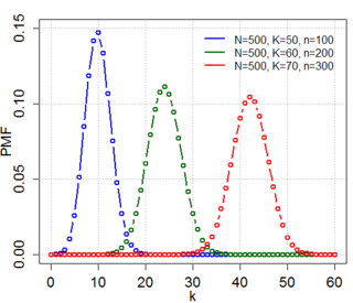
In probability theory and statistics, the hypergeometric distribution is a discrete probability distribution that describes the probability of successes in draws, without replacement, from a finite population of size that contains exactly objects with that feature, wherein each draw is either a success or a failure. In contrast, the binomial distribution describes the probability of successes in draws with replacement.

Pearson's chi-squared test or Pearson's test is a statistical test applied to sets of categorical data to evaluate how likely it is that any observed difference between the sets arose by chance. It is the most widely used of many chi-squared tests – statistical procedures whose results are evaluated by reference to the chi-squared distribution. Its properties were first investigated by Karl Pearson in 1900. In contexts where it is important to improve a distinction between the test statistic and its distribution, names similar to Pearson χ-squared test or statistic are used.

<span class="mw-page-title-main">Chi-squared test</span> Statistical hypothesis test

A chi-squared test is a statistical hypothesis test used in the analysis of contingency tables when the sample sizes are large. In simpler terms, this test is primarily used to examine whether two categorical variables are independent in influencing the test statistic. The test is valid when the test statistic is chi-squared distributed under the null hypothesis, specifically Pearson's chi-squared test and variants thereof. Pearson's chi-squared test is used to determine whether there is a statistically significant difference between the expected frequencies and the observed frequencies in one or more categories of a contingency table. For contingency tables with smaller sample sizes, a Fisher's exact test is used instead.

<span class="mw-page-title-main">Hardy–Weinberg principle</span> Principle in genetics

In population genetics, the Hardy–Weinberg principle, also known as the Hardy–Weinberg equilibrium, model, theorem, or law, states that allele and genotype frequencies in a population will remain constant from generation to generation in the absence of other evolutionary influences. These influences include genetic drift, mate choice, assortative mating, natural selection, sexual selection, mutation, gene flow, meiotic drive, genetic hitchhiking, population bottleneck, founder effect,inbreeding and outbreeding depression.

An odds ratio (OR) is a statistic that quantifies the strength of the association between two events, A and B. The odds ratio is defined as the ratio of the odds of A in the presence of B and the odds of A in the absence of B, or equivalently, the ratio of the odds of B in the presence of A and the odds of B in the absence of A. Two events are independent if and only if the OR equals 1, i.e., the odds of one event are the same in either the presence or absence of the other event. If the OR is greater than 1, then A and B are associated (correlated) in the sense that, compared to the absence of B, the presence of B raises the odds of A, and symmetrically the presence of A raises the odds of B. Conversely, if the OR is less than 1, then A and B are negatively correlated, and the presence of one event reduces the odds of the other event.

In null-hypothesis significance testing, the -value is the probability of obtaining test results at least as extreme as the result actually observed, under the assumption that the null hypothesis is correct. A very small p-value means that such an extreme observed outcome would be very unlikely under the null hypothesis. Even though reporting p-values of statistical tests is common practice in academic publications of many quantitative fields, misinterpretation and misuse of p-values is widespread and has been a major topic in mathematics and metascience. In 2016, the American Statistical Association (ASA) made a formal statement that "p-values do not measure the probability that the studied hypothesis is true, or the probability that the data were produced by random chance alone" and that "a p-value, or statistical significance, does not measure the size of an effect or the importance of a result" or "evidence regarding a model or hypothesis." That said, a 2019 task force by ASA has issued a statement on statistical significance and replicability, concluding with: "p-values and significance tests, when properly applied and interpreted, increase the rigor of the conclusions drawn from data."

In statistics, G-tests are likelihood-ratio or maximum likelihood statistical significance tests that are increasingly being used in situations where chi-squared tests were previously recommended.

In statistics, a contingency table is a type of table in a matrix format that displays the multivariate frequency distribution of the variables. They are heavily used in survey research, business intelligence, engineering, and scientific research. They provide a basic picture of the interrelation between two variables and can help find interactions between them. The term contingency table was first used by Karl Pearson in "On the Theory of Contingency and Its Relation to Association and Normal Correlation", part of the Drapers' Company Research Memoirs Biometric Series I published in 1904.

In statistics, the binomial test is an exact test of the statistical significance of deviations from a theoretically expected distribution of observations into two categories using sample data.

In probability theory, the multinomial distribution is a generalization of the binomial distribution. For example, it models the probability of counts for each side of a k-sided dice rolled n times. For n independent trials each of which leads to a success for exactly one of k categories, with each category having a given fixed success probability, the multinomial distribution gives the probability of any particular combination of numbers of successes for the various categories.

This glossary of statistics and probability is a list of definitions of terms and concepts used in the mathematical sciences of statistics and probability, their sub-disciplines, and related fields. For additional related terms, see Glossary of mathematics and Glossary of experimental design.

A permutation test is an exact statistical hypothesis test making use of the proof by contradiction. A permutation test involves two or more samples. The null hypothesis is that all samples come from the same distribution . Under the null hypothesis, the distribution of the test statistic is obtained by calculating all possible values of the test statistic under possible rearrangements of the observed data. Permutation tests are, therefore, a form of resampling.

Exact (significance) test is a test such that if the null hypothesis is true, then all assumptions made during the derivation of the distribution of the test statistic are met. Using an exact test provides a significance test that maintains the type I error rate of the test at the desired significance level of the test. For example, an exact test at a significance level of , when repeated over many samples where the null hypothesis is true, will reject at most of the time. This is in contrast to an approximate test in which the desired type I error rate is only approximately maintained, while this approximation may be made as close to as desired by making the sample size sufficiently large.

In combinatorics, the twelvefold way is a systematic classification of 12 related enumerative problems concerning two finite sets, which include the classical problems of counting permutations, combinations, multisets, and partitions either of a set or of a number. The idea of the classification is credited to Gian-Carlo Rota, and the name was suggested by Joel Spencer.

McNemar's test is a statistical test used on paired nominal data. It is applied to 2 × 2 contingency tables with a dichotomous trait, with matched pairs of subjects, to determine whether the row and column marginal frequencies are equal. It is named after Quinn McNemar, who introduced it in 1947. An application of the test in genetics is the transmission disequilibrium test for detecting linkage disequilibrium.

<span class="mw-page-title-main">Fisher's noncentral hypergeometric distribution</span>

In probability theory and statistics, Fisher's noncentral hypergeometric distribution is a generalization of the hypergeometric distribution where sampling probabilities are modified by weight factors. It can also be defined as the conditional distribution of two or more binomially distributed variables dependent upon their fixed sum.

In statistics, Barnard’s test is an exact test used in the analysis of 2 × 2 contingency tables with one margin fixed. Barnard’s tests are really a class of hypothesis tests, also known as unconditional exact tests for two independent binomials. These tests examine the association of two categorical variables and are often a more powerful alternative than Fisher's exact test for 2 × 2 contingency tables. While first published in 1945 by G.A. Barnard, the test did not gain popularity due to the computational difficulty of calculating the p value and Fisher’s specious disapproval. Nowadays, even for sample sizes n ~ 1 million, computers can often implement Barnard’s test in a few seconds or less.

Boschloo's test is a statistical hypothesis test for analysing 2x2 contingency tables. It examines the association of two Bernoulli distributed random variables and is a uniformly more powerful alternative to Fisher's exact test. It was proposed in 1970 by R. D. Boschloo.

References

  1. Fisher, R. A. (1922). "On the interpretation of χ2 from contingency tables, and the calculation of P". Journal of the Royal Statistical Society . 85 (1): 87–94. doi:10.2307/2340521. JSTOR   2340521.
  2. Fisher, R.A. (1954). Statistical Methods for Research Workers. Oliver and Boyd. ISBN   0-05-002170-2.
  3. Agresti, Alan (1992). "A Survey of Exact Inference for Contingency Tables". Statistical Science. 7 (1): 131–153. CiteSeerX   10.1.1.296.874 . doi:10.1214/ss/1177011454. JSTOR   2246001.
  4. Fisher, Sir Ronald A. (1956) [ The Design of Experiments (1935)]. "Mathematics of a Lady Tasting Tea". In James Roy Newman (ed.). The World of Mathematics, volume 3. Courier Dover Publications. ISBN   978-0-486-41151-4.
  5. Larntz, Kinley (1978). "Small-sample comparisons of exact levels for chi-squared goodness-of-fit statistics". Journal of the American Statistical Association. 73 (362): 253–263. doi:10.2307/2286650. JSTOR   2286650.
  6. Mehta, Cyrus R; Patel, Nitin R; Tsiatis, Anastasios A (1984). "Exact significance testing to establish treatment equivalence with ordered categorical data". Biometrics. 40 (3): 819–825. doi:10.2307/2530927. JSTOR   2530927. PMID   6518249.
  7. Mehta, C. R. 1995. SPSS 6.1 Exact test for Windows. Englewood Cliffs, NJ: Prentice Hall.
  8. Mehta C.R.; Patel N.R. (1983). "A Network Algorithm for Performing Fisher's Exact Test in r Xc Contingency Tables". Journal of the American Statistical Association. 78 (382): 427–434. doi:10.2307/2288652. JSTOR   2288652.
  9. mathworld.wolfram.com Page giving the formula for the general form of Fisher's exact test for m × n contingency tables
  10. Cyrus R. Mehta; Nitin R. Patel (1986). "ALGORITHM 643: FEXACT: a FORTRAN subroutine for Fisher's exact test on unordered r×c contingency tables". ACM Trans. Math. Softw. 12 (2): 154–161. doi: 10.1145/6497.214326 . S2CID   207666979.
  11. Mi, Huaiyu; Muruganujan, Anushya; Casagrande, John T.; Thomas, Paul D. (2013). "Large-scale gene function analysis with the PANTHER classification system". Nature Protocols. 8 (8): 1551–1566. doi:10.1038/nprot.2013.092. PMC   6519453 . PMID   23868073.
  12. STAT 226: Lecture 7, Section 2.6, Fisher’s Exact Tests. Yibi Huang, University of Chicago
  13. 1 2 Liddell, Douglas (1976). "Practical tests of 2×2 contingency tables". The Statistician. 25 (4): 295–304. doi:10.2307/2988087. JSTOR   2988087.
  14. 1 2 Berkson, Joseph (1978). "In dispraise of the exact test". Journal of Statistical Planning and Inference. 2: 27–42. doi:10.1016/0378-3758(78)90019-8.
  15. 1 2 D'Agostino, R. B.; Chase, W. & Belanger, A. (1988). "The appropriateness of some common procedures for testing equality of two independent binomial proportions". The American Statistician. 42 (3): 198–202. doi:10.2307/2685002. JSTOR   2685002.
  16. 1 2 3 4 Yates, F. (1984). "Tests of significance for 2 × 2 contingency tables (with discussion)". Journal of the Royal Statistical Society, Series A. 147 (3): 426–463. doi:10.2307/2981577. JSTOR   2981577. S2CID   15760519.
  17. 1 2 3 4 Little, Roderick J. A. (1989). "Testing the equality of two independent binomial proportions". The American Statistician. 43 (4): 283–288. doi:10.2307/2685390. JSTOR   2685390.
  18. Mehta, Cyrus R.; Senchaudhuri, Pralay (4 September 2003). "Conditional versus unconditional exact tests for comparing two binomials" (PDF). Retrieved 20 November 2009.
  19. Barnard, G.A. (1945). "A new test for 2×2 tables". Nature. 156 (3954): 177. Bibcode:1945Natur.156..177B. doi: 10.1038/156177a0 .
  20. 1 2 Fisher (1945). "A New Test for 2 × 2 Tables". Nature. 156 (3961): 388. Bibcode:1945Natur.156..388F. doi: 10.1038/156388a0 . S2CID   4113420.; Barnard, G.A. (1945). "A new test for 2×2 tables". Nature. 156 (3974): 783–784. Bibcode:1945Natur.156..783B. doi:10.1038/156783b0. S2CID   4099311.
  21. 1 2 3 4 Choi L, Blume JD, Dupont WD (2015). "Elucidating the foundations of statistical inference with 2×2 tables". PLOS ONE. 10 (4): e0121263. Bibcode:2015PLoSO..1021263C. doi: 10.1371/journal.pone.0121263 . PMC   4388855 . PMID   25849515.
  22. Lydersen, S., Fagerland, M. W., and Laake, P. (2009). "Recommended tests for association in 2× 2 tables". Statistics in Medicine. 28 (7): 1159–1175. doi:10.1002/sim.3531. PMID   19170020. S2CID   3900997.{{cite journal}}: CS1 maint: multiple names: authors list (link)
  23. Berger R.L. (1994). "Power comparison of exact unconditional tests for comparing two binomial proportions". Institute of Statistics Mimeo Series No. 2266: 1–19.
  24. Boschloo R.D. (1970). "Raised Conditional Level of Significance for the 2x2-table when Testing the Equality of Two Probabilities". Statistica Neerlandica. 24: 1–35. doi:10.1111/j.1467-9574.1970.tb00104.x.
  25. Choi, Leena (2011). "ProfileLikelihood: profile likelihood for a parameter in commonly used statistical models; 2011. R package version 1.1". See also: Likelihood Ratio Statistics for 2 x 2 Tables Archived 4 June 2016 at the Wayback Machine (Online calculator).