Backward induction is the process of determining a sequence of optimal choices by reasoning from the end point of a problem or situation back to its beginning via individual events or actions (point by point).[1] Backward induction involves examining the final point in a series of decisions and identifying the most optimal process or action required to arrive at that point. This process continues backward until the best action for every possible point along the sequence (i.e. for every possible information set) is determined. Backward induction was first utilized in 1875 by Arthur Cayley, who discovered the method while attempting to solve the secretary problem.[2]
In game theory, a variant of backward induction is a method used to compute subgame perfect equilibria in sequential games.[5] The difference is that optimization problems involve one decision maker who chooses what to do at each point of time, whereas game theory problems involve the decisions of several players interacting. In this situation it may still be possible to apply a generalization of backward induction, since by anticipating what the last player will do in each situation, it may be possible to determine what the second-to-last player will do, and so on. This variant of backward induction has been used to solve formal games from the very beginning of game theory. John von Neumann and Oskar Morgenstern suggested solving zero-sum, two-person formal games by this method in their Theory of Games and Economic Behavior (1944), the book which established game theory as a field of study.[6][7]
Decision making example
Optimal-stopping problem
A person facing ten years for potential employment opportunities (denoted as times 1, 2, ... 10) may encounter a choice between two job options: a 'good' job offering a salary of $100 or a 'bad' job providing a salary of $44. Each job type has an equal probability of being offered. Upon accepting a job, the individual will remain in that particular job for the entire remainder of the ten-year duration.
This scenario is simplified by assuming that the individual's entire concern is their total expected monetary earnings, without any variable preferences for earnings across different periods. In economic terms, this is a scenario with an implicit interest rate of zero and a constant marginal utility of money.
Whether the person in question should accept a 'bad' job can be decided by reasoning backwards from time 10.
At time 10, the total earnings from accepting a 'good' job is $100; the value of accepting a 'bad' job is $44; the total earnings from rejecting the available job is $0. Therefore, if they are still unemployed in the last period, they should accept whatever job they are offered at that time for greater income.
At time 9, the total earnings from accepting a 'good' job is 2 * $100 = $200 because that job will last for two years. The total earnings from accepting a 'bad' job is 2 * $44 = $88. The total expected earnings from rejecting a job offer are $0 now plus the value of the next job offer, which will either be $44 with 1/2 probability or $100 with 1/2 probability, for an average ('expected') value of ($100 + $44) / 2 = $72. Therefore, regardless of whether the job available at time 9 is 'good' or 'bad', they should accept it for greater income.
At time 8, the total earnings from accepting a 'good' job is 3 * $100 = $300 (it will last for three years); the total earnings from accepting a 'bad' job is 3 * $44 = $132. The total expected earnings from rejecting a job offer is $0 now plus the total expected earnings from waiting for a job offer at a time t=9. As concluded above, any offer at time 9 should be accepted and the expected value of doing so is ($200 + $88) / 2 = $144. Therefore, at time 8, total expected earnings are higher if the person waits for the next offer rather than accepting a 'bad' job.
It can be verified by continuing to work backwards that a 'bad' offer should only be accepted if the person is still unemployed at time 9 or time 10; a bad offer should be rejected at any time up through time 8. Generalizing this example intuitively, it corresponds to the principle that if one expects to work in a job for a long time, it is worth picking carefully.
A dynamic optimization problem of this kind is called an optimal stopping problem because the issue at hand is when to stop waiting for a better offer. Search theory is a field of microeconomics that applies models of this type to matters such as shopping, job searches, and marriage.
Game theory
In game theory, backward induction is a solution concept that follows from applying sequential rationality to identify an optimal action for each information set in a given game tree. It develops the implications of rationality via individual information sets in the extensive-form representation of a game.[8]
In order to solve for a subgame perfect equilibrium with backwards induction, the game should be written out in extensive form and then divided into subgames. Starting with the subgame furthest from the initial node, or starting point, the expected payoffs listed for this subgame are weighed, and a rational player will select the option with the higher payoff for themselves. The highest payoff vector is selected and marked. To solve for the subgame perfect equilibrium, one should continually work backwards from subgame to subgame until one arrives at the starting point. As this process progresses, the initial extensive form game will become shorter and shorter. The marked path of vectors is the subgame perfect equilibrium.[9]
This idea of backward induction in game theory can be demonstrated with a simple example.
Multi-stage game
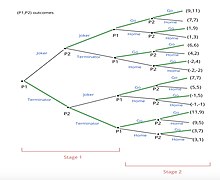
A natural first example is a multi-stage game involving 2 players. Players are planning to go to a movie. Currently, 2 movies are very popular, Joker and Terminator. Player 1 wants to watch Terminator, and Player 2 wants to watch Joker. Player 1 will buy a ticket first and tell Player 2 about her choice. Then, Player 2 will buy his ticket. Once they both observe the choices, in the second stage, they choose whether to go to the movie or stay home. Just like in the first stage, Player 1 chooses first, then Player 2 makes his choice after observing Player 1's choice.
For this example, payoffs are added across different stages. The game is a perfect information game.
Steps for solving this Multi-Stage Game, with the extensive form as seen to the right:
Backward induction starts solving the game from the final nodes.
Player 2 will observe 8 subgames from the final nodes to choose "Go to Movie" or "Stay Home."
Player 2 would make 4 possible comparisons in total. In each case he would choose the option with the highest payoff.
For example, considering the first subgame, payoff of 11 is higher than 7. Therefore, Player 2 would choose "Go to Movie."
The method continues for every subgame.
Once one has determined how Player 2 would choose, one analyzes Player 1's prior choices based on selected subgames.
The process is similar to Step 2. One compares Player 1's payoffs in order to anticipate her choices.
Subgames that would not be chosen by Player 2 in the previous step are no longer considered because they are ruled out by the assumption of rational play.
For example, the choice "Go to Movie" offers a payoff of 9 (9,11) and the choice "Stay Home" offers a payoff of 1 (1, 9). Player 1 would choose "Go to Movie."
The process repeats for each player until the initial node is reached.
For example, Player 2 would choose "Joker" because a payoff of 11 (9, 11) is greater than "Terminator" with a payoff of 6 (6, 6).
For example, Player 1, at initial node, would select "Terminator" because it offers a higher payoff of 11. Terminator: (11, 9) > Joker: (9, 11).
To identify a subgame perfect equilibrium, one needs to identify a route that selects an optimal subgame at each information set.
In this example, Player 1 chooses "Terminator" and Player 2 also chooses "Terminator." Then they both choose "Go to Movie."
The subgame perfect equilibrium leads to a payoff of (11,9).
Limitations
Backward induction can be applied to only limited classes of games. The procedure is well-defined for any game of perfect information with no ties of utility. It is also well-defined and meaningful for games of perfect information with ties. However, in such cases it leads to more than one perfect strategy. The procedure can be applied to some games with nontrivial information sets, but it is not applicable in general. It is best suited to solve games with perfect information. If all players are not aware of the other players' actions and payoffs at each decision node, then backward induction is not so easily applied.[10]
Furthermore, even in games that formally allow for backward induction in theory, it may not accurately predict empirical game play in practice. This can be demonstrated with a second example.
A second, more famous example of an asymmetric game consists of two players: Player 1 proposes to split a dollar with Player 2, which Player 2 then accepts or rejects. This is called the ultimatum game. Player 1 acts first by splitting the dollar however they see fit. Next, Player 2 either accepts the portion they have been offered by Player 1 or rejects the split. If Player 2 accepts the split, then both Player 1 and Player 2 get the payoffs matching that split. If Player 2 decides to reject Player 1's offer, then both players get nothing. In other words, Player 2 has veto power over Player 1's proposed allocation, but applying the veto eliminates any reward for both players.[11]
Considering the choice and response of Player 2 given any arbitrary proposal by Player 1, formal rationality prescribes that Player 2 would accept any payoff that is greater than or equal to $0. Accordingly, by backward induction Player 1 ought to propose giving Player 2 as little as possible in order to gain the largest portion of the split. Player 1 giving Player 2 the smallest unit of money and keeping the rest for themselves is the unique subgame-perfect equilibrium. The ultimatum game does have several other Nash Equilibria which are not subgame perfect and therefore do not arise via backward induction.
The ultimatum game is a theoretical illustration of the usefulness of backward induction when considering infinite games, but the ultimatum game's theoretically predicted results do not match empirical observation. Experimental evidence has shown that a proposer, Player 1, very rarely offers $0 and the responder, Player 2, sometimes rejects offers greater than $0. What is deemed acceptable by Player 2 varies with context. The pressure or presence of other players and external implications can mean that the game's formal model cannot necessarily predict what a real person will choose. According to Colin Camerer, an American behavioral economist, Player 2 "rejects offers of less than 20 percent of X about half the time, even though they end up with nothing."[12]
While backward induction assuming formal rationality would predict that a responder would accept any offer greater than zero, responders in reality are not formally rational players and therefore often seem to care more about offer 'fairness' or perhaps other anticipations of indirect or external effects rather than immediate potential monetary gains.
Economics
Entry-decision problem
A dynamic game in which the players are an incumbent firm in an industry and a potential entrant to that industry is to be considered. As it stands, the incumbent has a monopoly over the industry and does not want to lose some of its market share to the entrant. If the entrant chooses not to enter, the payoff to the incumbent is high (it maintains its monopoly) and the entrant neither loses nor gains (its payoff is zero). If the entrant enters, the incumbent can "fight" or "accommodate" the entrant. It will fight by lowering its price, running the entrant out of business (and incurring exit costs — a negative payoff) and damaging its own profits. If it accommodates the entrant it will lose some of its sales, but a high price will be maintained and it will receive greater profits than by lowering its price (but lower than monopoly profits).
If the incumbent accommodates given the case that the entrant enters, the best response for the entrant is to enter (and gain profit). Hence the strategy profile in which the entrant enters and the incumbent accommodates if the entrant enters is a Nash equilibrium consistent with backward induction. However, if the incumbent is going to fight, the best response for the entrant is to not enter, and if the entrant does not enter, it does not matter what the incumbent chooses to do in the hypothetical case that the entrant does enter. Hence the strategy profile in which the incumbent fights if the entrant enters, but the entrant does not enter is also a Nash equilibrium. However, were the entrant to deviate and enter, the incumbent's best response is to accommodate—the threat of fighting is not credible. This second Nash equilibrium can therefore be eliminated by backward induction.
Finding a Nash equilibrium in each decision-making process (subgame) constitutes as perfect subgame equilibria. Thus, these strategy profiles that depict subgame perfect equilibria exclude the possibility of actions like incredible threats that are used to "scare off" an entrant. If the incumbent threatens to start a price war with an entrant, they are threatening to lower their prices from a monopoly price to slightly lower than the entrant's, which would be impractical, and incredible, if the entrant knew a price war would not actually happen since it would result in losses for both parties. Unlike a single agent optimization which includes equilibria that aren't feasible or optimal, a subgame perfect equilibrium accounts for the actions of another player, thus ensuring that no player reaches a subgame mistakenly. In this case, backwards induction yielding perfect subgame equilibria ensures that the entrant will not be convinced of the incumbent's threat knowing that it was not a best response in the strategy profile.[13]
The unexpected hanging paradox is a paradox related to backward induction. The prisoner described in the paradox uses backwards induction to reach a false conclusion. The description of the problem assumes it is possible to surprise someone who is performing backward induction. The mathematical theory of backward induction does not make this assumption, so the paradox does not call into question the results of this theory.
Common knowledge of rationality
Backward induction works only if both players are rational, i.e., always select an action that maximizes their payoff. However, rationality is not enough: each player should also believe that all other players are rational. Even this is not enough: each player should believe that all other players know that all other players are rational, and so on, ad infinitum. In other words, rationality should be common knowledge.[14]
Limited backward induction
Limited backward induction is a deviation from fully rational backward induction. It involves enacting the regular process of backward induction without perfect foresight. Theoretically, this occurs when one or more players have limited foresight and cannot perform backward induction through all terminal nodes.[15] Limited backward induction plays a much larger role in longer games as the effects of limited backward induction are more potent in later periods of games.
A four-stage sequential game with a foresight bound
Experiments have shown that in sequential bargaining games, such as the Centipede game, subjects deviate from theoretical predictions and instead engage in limited backward induction. This deviation occurs as a result of bounded rationality, where players can only perfectly see a few stages ahead.[16] This allows for unpredictability in decisions and inefficiency in finding and achieving subgame perfect Nash equilibria.
There are three broad hypotheses for this phenomenon:
The presence of social factors (e.g. fairness)
The presence of non-social factors (e.g. limited backward induction)
Cultural difference
Violations of backward induction is predominantly attributed to the presence of social factors. However, data-driven model predictions for sequential bargaining games (using the cognitive hierarchy model) have highlighted that in some games the presence of limited backward induction can play a dominant role.[17]
Within repeated public goods games, team behavior is impacted by limited backward induction; where it is evident that team members' initial contributions are higher than contributions towards the end. Limited backward induction also influences how regularly free-riding occurs within a team's public goods game. Early on, when the effects of limited backward induction are low, free-riding is less frequent, whilst towards the end, when effects are high, free-riding becomes more frequent.[18]
Limited backward induction has also been tested for within a variant of the race game. In the game, players would sequentially choose integers inside a range and sum their choices until a target number is reached. Hitting the target earns that player a prize; the other loses. Partway through a series of games, a small prize was introduced. The majority of players then performed limited backward induction, as they solved for the small prize rather than for the original prize. Only a small fraction of players considered both prizes at the start.[19]
Most tests of backward induction are based on experiments, in which participants are only to a small extent incentivized to perform the task well, if at all. However, violations of backward induction also appear to be common in high-stakes environments. A large-scale analysis of the American television game show The Price Is Right, for example, provides evidence of limited foresight. In every episode, contestants play the Showcase Showdown, a sequential game of perfect information for which the optimal strategy can be found through backward induction. The frequent and systematic deviations from optimal behavior suggest that a sizable proportion of the contestants fail to properly backward induct and myopically consider the next stage of the game only.[20]
↑ Rust J. (2008) Dynamic Programming. In: Palgrave Macmillan (eds) The New Palgrave Dictionary of Economics. Palgrave Macmillan, London
↑ Aumann, Robert J. (January 1995). "Backward induction and common knowledge of rationality". Games and Economic Behavior. 8 (1): 6–19. doi:10.1016/S0899-8256(05)80015-6.
↑ Marco Mantovani, 2015. "Limited backward induction: foresight and behavior in sequential games," Working Papers 289, University of Milano-Bicocca, Department of Economics
↑ Qu, Xia; Doshi, Prashant (1 March 2017). "On the role of fairness and limited backward induction in sequential bargaining games". Annals of Mathematics and Artificial Intelligence. 79 (1): 205–227. doi:10.1007/s10472-015-9481-7. S2CID23565130.
↑ Cox, Caleb A.; Stoddard, Brock (May 2018). "Strategic thinking in public goods games with teams". Journal of Public Economics. 161: 31–43. doi:10.1016/j.jpubeco.2018.03.007.
In game theory, the Nash equilibrium is the most commonly-used solution concept for non-cooperative games. A Nash equilibrium is a situation where no player could gain by changing their own strategy. The idea of Nash equilibrium dates back to the time of Cournot, who in 1838 applied it to his model of competition in an oligopoly.
The ultimatum game is a game that has become a popular instrument of economic experiments. An early description is by Nobel laureate John Harsanyi in 1961. One player, the proposer, is endowed with a sum of money. The proposer is tasked with splitting it with another player, the responder. Once the proposer communicates their decision, the responder may accept it or reject it. If the responder accepts, the money is split per the proposal; if the responder rejects, both players receive nothing. Both players know in advance the consequences of the responder accepting or rejecting the offer.
In game theory, the centipede game, first introduced by Robert Rosenthal in 1981, is an extensive form game in which two players take turns choosing either to take a slightly larger share of an increasing pot, or to pass the pot to the other player. The payoffs are arranged so that if one passes the pot to one's opponent and the opponent takes the pot on the next round, one receives slightly less than if one had taken the pot on this round, but after an additional switch the potential payoff will be higher. Therefore, although at each round a player has an incentive to take the pot, it would be better for them to wait. Although the traditional centipede game had a limit of 100 rounds, any game with this structure but a different number of rounds is called a centipede game.
In game theory, a player's strategy is any of the options which they choose in a setting where the optimal outcome depends not only on their own actions but on the actions of others. The discipline mainly concerns the action of a player in a game affecting the behavior or actions of other players. Some examples of "games" include chess, bridge, poker, monopoly, diplomacy or battleship. A player's strategy will determine the action which the player will take at any stage of the game. In studying game theory, economists enlist a more rational lens in analyzing decisions rather than the psychological or sociological perspectives taken when analyzing relationships between decisions of two or more parties in different disciplines.
In game theory, a solution concept is a formal rule for predicting how a game will be played. These predictions are called "solutions", and describe which strategies will be adopted by players and, therefore, the result of the game. The most commonly used solution concepts are equilibrium concepts, most famously Nash equilibrium.
In game theory, an extensive-form game is a specification of a game allowing for the explicit representation of a number of key aspects, like the sequencing of players' possible moves, their choices at every decision point, the information each player has about the other player's moves when they make a decision, and their payoffs for all possible game outcomes. Extensive-form games also allow for the representation of incomplete information in the form of chance events modeled as "moves by nature". Extensive-form representations differ from normal-form in that they provide a more complete description of the game in question, whereas normal-form simply boils down the game into a payoff matrix.
In game theory, a Perfect Bayesian Equilibrium (PBE) is a solution with Bayesian probability to a turn-based game with incomplete information. More specifically, it is an equilibrium concept that uses Bayesian updating to describe player behavior in dynamic games with incomplete information. Perfect Bayesian equilibria are used to solve the outcome of games where players take turns but are unsure of the "type" of their opponent, which occurs when players don't know their opponent's preference between individual moves. A classic example of a dynamic game with types is a war game where the player is unsure whether their opponent is a risk-taking "hawk" type or a pacifistic "dove" type. Perfect Bayesian Equilibria are a refinement of Bayesian Nash equilibrium (BNE), which is a solution concept with Bayesian probability for non-turn-based games.
In game theory, a sequential game is a game where one player chooses their action before the others choose theirs. The other players must have information on the first player's choice so that the difference in time has no strategic effect. Sequential games are governed by the time axis and represented in the form of decision trees.
The chain store paradox is an apparent game theory paradox describing the decisions a chain store might make, where a "deterrence strategy" appears optimal instead of the backward induction strategy of standard game theory reasoning.
In game theory, trembling hand perfect equilibrium is a type of refinement of a Nash equilibrium that was first proposed by Reinhard Selten. A trembling hand perfect equilibrium is an equilibrium that takes the possibility of off-the-equilibrium play into account by assuming that the players, through a "slip of the hand" or tremble, may choose unintended strategies, albeit with negligible probability.
In game theory, folk theorems are a class of theorems describing an abundance of Nash equilibrium payoff profiles in repeated games. The original Folk Theorem concerned the payoffs of all the Nash equilibria of an infinitely repeated game. This result was called the Folk Theorem because it was widely known among game theorists in the 1950s, even though no one had published it. Friedman's (1971) Theorem concerns the payoffs of certain subgame-perfect Nash equilibria (SPE) of an infinitely repeated game, and so strengthens the original Folk Theorem by using a stronger equilibrium concept: subgame-perfect Nash equilibria rather than Nash equilibria.
In game theory, a repeated game is an extensive form game that consists of a number of repetitions of some base game. The stage game is usually one of the well-studied 2-person games. Repeated games capture the idea that a player will have to take into account the impact of their current action on the future actions of other players; this impact is sometimes called their reputation. Single stage game or single shot game are names for non-repeated games.
In game theory, a Manipulated Nash equilibrium or MAPNASH is a refinement of subgame perfect equilibrium used in dynamic games of imperfect information. Informally, a strategy set is a MAPNASH of a game if it would be a subgame perfect equilibrium of the game if the game had perfect information. MAPNASH were first suggested by Amershi, Sadanand, and Sadanand (1988) and has been discussed in several papers since. It is a solution concept based on how players think about other players' thought processes.
In game theory, a subgame perfect equilibrium is a refinement of a Nash equilibrium used in dynamic games. A strategy profile is a subgame perfect equilibrium if it represents a Nash equilibrium of every subgame of the original game. Informally, this means that at any point in the game, the players' behavior from that point onward should represent a Nash equilibrium of the continuation game, no matter what happened before. Every finite extensive game with perfect recall has a subgame perfect equilibrium. Perfect recall is a term introduced by Harold W. Kuhn in 1953 and "equivalent to the assertion that each player is allowed by the rules of the game to remember everything he knew at previous moves and all of his choices at those moves".
Quantal response equilibrium (QRE) is a solution concept in game theory. First introduced by Richard McKelvey and Thomas Palfrey, it provides an equilibrium notion with bounded rationality. QRE is not an equilibrium refinement, and it can give significantly different results from Nash equilibrium. QRE is only defined for games with discrete strategies, although there are continuous-strategy analogues.
A non-credible threat is a term used in game theory and economics to describe a threat in a sequential game that a rational player would not actually carry out, because it would not be in his best interest to do so.
A Markov perfect equilibrium is an equilibrium concept in game theory. It has been used in analyses of industrial organization, macroeconomics, and political economy. It is a refinement of the concept of subgame perfect equilibrium to extensive form games for which a pay-off relevant state space can be identified. The term appeared in publications starting about 1988 in the work of economists Jean Tirole and Eric Maskin.
Jean-François Mertens was a Belgian game theorist and mathematical economist.
In game theory, Mertens stability is a solution concept used to predict the outcome of a non-cooperative game. A tentative definition of stability was proposed by Elon Kohlberg and Jean-François Mertens for games with finite numbers of players and strategies. Later, Mertens proposed a stronger definition that was elaborated further by Srihari Govindan and Mertens. This solution concept is now called Mertens stability, or just stability.
This page is based on this Wikipedia article Text is available under the CC BY-SA 4.0 license; additional terms may apply. Images, videos and audio are available under their respective licenses.