Bi-elliptic transfer

Last updated
A bi-elliptic transfer from a low circular starting orbit (blue) to a higher circular orbit (red) Bi-elliptic transfer.svg
A bi-elliptic transfer from a low circular starting orbit (blue) to a higher circular orbit (red)
Comparable Hohmann transfer orbit (2), from a low circular orbit (1) to a higher orbit (3) Hohmann transfer orbit.svg
Comparable Hohmann transfer orbit (2), from a low circular orbit (1) to a higher orbit (3)

In astronautics and aerospace engineering, the bi-elliptic transfer is an orbital maneuver that moves a spacecraft from one orbit to another and may, in certain situations, require less delta-v than a Hohmann transfer maneuver.

Contents

The bi-elliptic transfer consists of two half-elliptic orbits. From the initial orbit, a first burn expends delta-v to boost the spacecraft into the first transfer orbit with an apoapsis at some point away from the central body. At this point a second burn sends the spacecraft into the second elliptical orbit with periapsis at the radius of the final desired orbit, where a third burn is performed, injecting the spacecraft into the desired orbit. [1]

While they require one more engine burn than a Hohmann transfer and generally require a greater travel time, some bi-elliptic transfers require a lower amount of total delta-v than a Hohmann transfer when the ratio of final to initial semi-major axis is 11.94 or greater, depending on the intermediate semi-major axis chosen. [2]

The idea of the bi-elliptical transfer trajectory was first[ citation needed ] published by Ary Sternfeld in 1934. [3]

Calculation

Delta-v

The three required changes in velocity can be obtained directly from the vis-viva equation

where

In what follows,

Starting from the initial circular orbit with radius (dark blue circle in the figure to the right), a prograde burn (mark 1 in the figure) puts the spacecraft on the first elliptical transfer orbit (aqua half-ellipse). The magnitude of the required delta-v for this burn is

When the apoapsis of the first transfer ellipse is reached at a distance from the primary, a second prograde burn (mark 2) raises the periapsis to match the radius of the target circular orbit, putting the spacecraft on a second elliptic trajectory (orange half-ellipse). The magnitude of the required delta-v for the second burn is

Lastly, when the final circular orbit with radius is reached, a retrograde burn (mark 3) circularizes the trajectory into the final target orbit (red circle). The final retrograde burn requires a delta-v of magnitude

If , then the maneuver reduces to a Hohmann transfer (in that case can be verified to become zero). Thus the bi-elliptic transfer constitutes a more general class of orbital transfers, of which the Hohmann transfer is a special two-impulse case.

A bi-parabolic transfer from a low circular starting orbit (dark blue) to a higher circular orbit (red) Bi-parabolicTransfer.png
A bi-parabolic transfer from a low circular starting orbit (dark blue) to a higher circular orbit (red)

The maximal possible savings can be computed by assuming that , in which case the total simplifies to . In this case, one also speaks of a bi-parabolic transfer because the two transfer trajectories are no longer ellipses but parabolas. The transfer time increases to infinity too.

Transfer time

Like the Hohmann transfer, both transfer orbits used in the bi-elliptic transfer constitute exactly one half of an elliptic orbit. This means that the time required to execute each phase of the transfer is half the orbital period of each transfer ellipse.

Using the equation for the orbital period and the notation from above,

The total transfer time is the sum of the times required for each half-orbit. Therefore:

and finally:

Comparison with the Hohmann transfer

Delta-v

Delta-v required for Hohmann (thick black curve) and bi-elliptic transfers (colored curves) between two circular orbits as a function of the ratio of their radii Bielliptic transfers comparison.svg
Delta-v required for Hohmann (thick black curve) and bi-elliptic transfers (colored curves) between two circular orbits as a function of the ratio of their radii

The figure shows the total required to transfer from a circular orbit of radius to another circular orbit of radius . The is shown normalized to the orbital speed in the initial orbit, , and is plotted as a function of the ratio of the radii of the final and initial orbits, ; this is done so that the comparison is general (i.e. not dependent of the specific values of and , only on their ratio). [2]

The thick black curve indicates the for the Hohmann transfer, while the thinner colored curves correspond to bi-elliptic transfers with varying values of the parameter , defined as the apoapsis radius of the elliptic auxiliary orbit normalized to the radius of the initial orbit, and indicated next to the curves. The inset shows a close-up of the region where the bi-elliptic curves cross the Hohmann curve for the first time.

One sees that the Hohmann transfer is always more efficient if the ratio of radii is smaller than 11.94. On the other hand, if the radius of the final orbit is more than 15.58 times larger than the radius of the initial orbit, then any bi-elliptic transfer, regardless of its apoapsis radius (as long as it's larger than the radius of the final orbit), requires less than a Hohmann transfer. Between the ratios of 11.94 and 15.58, which transfer is best depends on the apoapsis distance . For any given in this range, there is a value of above which the bi-elliptic transfer is superior and below which the Hohmann transfer is better. The following table lists the value of that results in the bi-elliptic transfer being better for some selected cases. [4]

Minimal such that a bi-elliptic transfer needs less [5]
Ratio of radii, Minimal Comments
<11.94N/AHohmann transfer is always better
11.94Bi-parabolic transfer
12815.81
1348.90
1426.10
1518.19
15.5815.58
>15.58Any bi-elliptic transfer is better

Transfer time

The long transfer time of the bi-elliptic transfer,

is a major drawback for this maneuver. It even becomes infinite for the bi-parabolic transfer limiting case.

The Hohmann transfer takes less than half of the time because there is just one transfer half-ellipse. To be precise,

Versatility in combination maneuvers

While a bi-elliptic transfer has a small parameter window where it's strictly superior to a Hohmann Transfer in terms of delta V for a planar transfer between circular orbits, the savings is fairly small, and a bi-elliptic transfer is a far greater aid when used in combination with certain other maneuvers.

At apoapsis, the spacecraft is travelling at low orbital velocity, and significant changes in periapsis can be achieved for small delta V cost. Transfers that resemble a bi-elliptic but which incorporate a plane-change maneuver at apoapsis can dramatically save delta-V on missions where the plane needs to be adjusted as well as the altitude, versus making the plane change in low circular orbit on top of a Hohmann transfer.

Likewise, dropping periapsis all the way into the atmosphere of a planetary body for aerobraking is inexpensive in velocity at apoapsis, but permits the use of "free" drag to aid in the final circularization burn to drop apoapsis; though it adds an extra mission stage of periapsis-raising back out of the atmosphere, this may, under some parameters, cost significantly less delta V than simply dropping periapsis in one burn from circular orbit.

Example

To transfer from a circular low Earth orbit with r0 = 6700 km to a new circular orbit with r1 = 93 800 km using a Hohmann transfer orbit requires a Δv of 2825.02 + 1308.70 = 4133.72 m/s. However, because r1 = 14r0> 11.94r0, it is possible to do better with a bi-elliptic transfer. If the spaceship first accelerated 3061.04 m/s, thus achieving an elliptic orbit with apogee at r2 = 40r0 = 268 000 km, then at apogee accelerated another 608.825 m/s to a new orbit with perigee at r1 = 93 800 km, and finally at perigee of this second transfer orbit decelerated by 447.662 m/s, entering the final circular orbit, then the total Δv would be only 4117.53 m/s, which is 16.19 m/s (0.4%) less.

The Δv saving could be further improved by increasing the intermediate apogee, at the expense of longer transfer time. For example, an apogee of 75.8r0 = 507 688 km (1.3 times the distance to the Moon) would result in a 1% Δv saving over a Hohmann transfer, but require a transit time of 17 days. As an impractical extreme example, an apogee of 1757r0 = 11 770 000 km (30 times the distance to the Moon) would result in a 2% Δv saving over a Hohmann transfer, but the transfer would require 4.5 years (and, in practice, be perturbed by the gravitational effects of other Solar system bodies). For comparison, the Hohmann transfer requires 15 hours and 34 minutes.

Δv for various orbital transfers
TypeHohmannBi-elliptic
Apogee (km)93 800268 000507 68811 770 000
Burn
(m/s)
1Increase2.svg 2825.02Increase2.svg 3061.04Increase2.svg 3123.62Increase2.svg 3191.79Increase2.svg 3194.89
2Increase2.svg 1308.70Increase2.svg 608.825Increase2.svg 351.836Increase2.svg 16.9336Steady2.svg 0
3Steady2.svg 0Decrease2.svg 447.662Decrease2.svg 616.926Decrease2.svg 842.322Decrease2.svg 853.870
Total (m/s)4133.724117.534092.384051.044048.76
Of Hohmann100%99.6%99.0%98.0%97.94%

Evidently, the bi-elliptic orbit spends more of its delta-v early on (in the first burn). This yields a higher contribution to the specific orbital energy and, due to the Oberth effect, is responsible for the net reduction in required delta-v.

See also

Related Research Articles

Orbit Curved path of an object around a point

In celestial mechanics, an orbit is the curved trajectory of an object such as the trajectory of a planet around a star, or of a natural satellite around a planet, or of an artificial satellite around an object or position in space such as a planet, moon, asteroid, or Lagrange point. Normally, orbit refers to a regularly repeating trajectory, although it may also refer to a non-repeating trajectory. To a close approximation, planets and satellites follow elliptic orbits, with the center of mass being orbited at a focal point of the ellipse, as described by Kepler's laws of planetary motion.

Hohmann transfer orbit Low-impulse transfer maneuver between two orbits of different altitudes

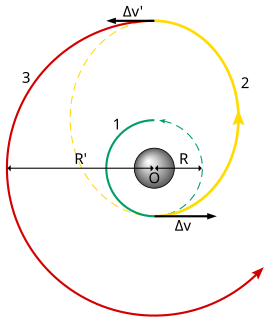
In astronautics, the Hohmann transfer orbit is an orbital maneuver used to transfer a spacecraft between two circular orbits of different altitudes around a central body. Examples would be used for travel between low Earth orbit and the Moon, or another solar planet or asteroid. It is accomplished by placing the craft into an elliptical orbit that is tangential to both the initial and target orbits in the same plane. The maneuver uses two engine impulses: the first prograde impulse places it on the transfer orbit by raising the craft's apoapsis to the target orbit's altitude; and the second raises the craft's periapsis to match the target orbit. The Hohmann maneuver often uses the lowest possible amount of impulse to accomplish the transfer, but requires a relatively longer travel time than higher-impulse transfers. In some cases, a bi-elliptic transfer can use even less impulse, but with a greater penalty in travel time.

Orbital mechanics Field of classical mechanics concerned with the motion of spacecraft

Orbital mechanics or astrodynamics is the application of ballistics and celestial mechanics to the practical problems concerning the motion of rockets and other spacecraft. The motion of these objects is usually calculated from Newton's laws of motion and law of universal gravitation. Orbital mechanics is a core discipline within space-mission design and control.

Orbital speed Speed at which a body orbits around the barycenter of a system

In gravitationally bound systems, the orbital speed of an astronomical body or object is the speed at which it orbits around either the barycenter or, if one object is much more massive than the other bodies in the system, its speed relative to the center of mass of the most massive body.

Sub-orbital spaceflight Spaceflight that does not complete an orbit around the earth

A sub-orbital spaceflight is a spaceflight in which the spacecraft reaches outer space, but its trajectory intersects the atmosphere or surface of the gravitating body from which it was launched, so that it will not complete one orbital revolution or reach escape velocity.

Delta-<i>v</i> budget

In astrodynamics and aerospace, a delta-v budget is an estimate of the total change in velocity (delta-v) required for a space mission. It is calculated as the sum of the delta-v required to perform each propulsive maneuver needed during the mission. As input to the Tsiolkovsky rocket equation, it determines how much propellant is required for a vehicle of given empty mass and propulsion system.

In spaceflight, an orbital maneuver is the use of propulsion systems to change the orbit of a spacecraft. For spacecraft far from Earth an orbital maneuver is called a deep-space maneuver (DSM).

Orbital inclination change is an orbital maneuver aimed at changing the inclination of an orbiting body's orbit. This maneuver is also known as an orbital plane change as the plane of the orbit is tipped. This maneuver requires a change in the orbital velocity vector at the orbital nodes.

Orbit phasing

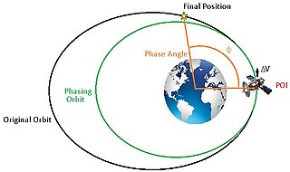
In astrodynamics, orbit phasing is the adjustment of the time-position of spacecraft along its orbit, usually described as adjusting the orbiting spacecraft's true anomaly. Orbital phasing is primarily used in scenarios where a spacecraft in a given orbit must be moved to a different location within the same orbit. The change in position within the orbit is usually defined as the phase angle, ϕ, and is the change in true anomaly required between the spacecraft's current position to the final position.

Parabolic trajectory

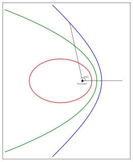
In astrodynamics or celestial mechanics a parabolic trajectory is a Kepler orbit with the eccentricity equal to 1 and is an unbound orbit that is exactly on the border between elliptical and hyperbolic. When moving away from the source it is called an escape orbit, otherwise a capture orbit. It is also sometimes referred to as a C3 = 0 orbit (see Characteristic energy).

Hyperbolic trajectory

In astrodynamics or celestial mechanics, a hyperbolic trajectory is the trajectory of any object around a central body with more than enough speed to escape the central object's gravitational pull. The name derives from the fact that according to Newtonian theory such an orbit has the shape of a hyperbola. In more technical terms this can be expressed by the condition that the orbital eccentricity is greater than one.

Elliptic orbit Kepler orbit with an eccentricity of less than one

In astrodynamics or celestial mechanics, an elliptic orbit or elliptical orbit is a Kepler orbit with an eccentricity of less than 1; this includes the special case of a circular orbit, with eccentricity equal to 0. In a stricter sense, it is a Kepler orbit with the eccentricity greater than 0 and less than 1. In a wider sense, it is a Kepler's orbit with negative energy. This includes the radial elliptic orbit, with eccentricity equal to 1.

Circular orbit Orbit with a fixed distance from the barycenter

A circular orbit is an orbit with a fixed distance around the barycenter; that is, in the shape of a circle.

Specific orbital energy

In the gravitational two-body problem, the specific orbital energy of two orbiting bodies is the constant sum of their mutual potential energy and their total kinetic energy, divided by the reduced mass. According to the orbital energy conservation equation, it does not vary with time:

In astrodynamics an orbit equation defines the path of orbiting body around central body relative to , without specifying position as a function of time. Under standard assumptions, a body moving under the influence of a force, directed to a central body, with a magnitude inversely proportional to the square of the distance, has an orbit that is a conic section with the central body located at one of the two foci, or the focus.

Vis-viva equation

In astrodynamics, the vis-viva equation, also referred to as orbital-energy-invariance law, is one of the equations that model the motion of orbiting bodies. It is the direct result of the principle of conservation of mechanical energy which applies when the only force acting on an object is its own weight.

Orbital eccentricity Amount by which an orbit deviates from a perfect circle

In astrodynamics, the orbital eccentricity of an astronomical object is a dimensionless parameter that determines the amount by which its orbit around another body deviates from a perfect circle. A value of 0 is a circular orbit, values between 0 and 1 form an elliptic orbit, 1 is a parabolic escape orbit, and greater than 1 is a hyperbola. The term derives its name from the parameters of conic sections, as every Kepler orbit is a conic section. It is normally used for the isolated two-body problem, but extensions exist for objects following a rosette orbit through the Galaxy.

Flight dynamics (spacecraft) Application of mechanical dynamics to model the flight of space vehicles

Spacecraft flight dynamics is the application of mechanical dynamics to model how the external forces acting on a space vehicle or spacecraft determine its flight path. These forces are primarily of three types: propulsive force provided by the vehicle's engines; gravitational force exerted by the Earth and other celestial bodies; and aerodynamic lift and drag.

Oberth effect Type of spacecraft maneuver

In astronautics, a powered flyby, or Oberth maneuver, is a maneuver in which a spacecraft falls into a gravitational well and then uses its engines to further accelerate as it is falling, thereby achieving additional speed. The resulting maneuver is a more efficient way to gain kinetic energy than applying the same impulse outside of a gravitational well. The gain in efficiency is explained by the Oberth effect, wherein the use of a reaction engine at higher speeds generates a greater change in mechanical energy than its use at lower speeds. In practical terms, this means that the most energy-efficient method for a spacecraft to burn its fuel is at the lowest possible orbital periapsis, when its orbital velocity is greatest. In some cases, it is even worth spending fuel on slowing the spacecraft into a gravity well to take advantage of the efficiencies of the Oberth effect. The maneuver and effect are named after the person who first described them in 1927, Hermann Oberth, an Austro-Hungarian-born German physicist and a founder of modern rocketry.

Semi-major and semi-minor axes Term in geometry; longest and shortest semidiameters of an ellipse

In geometry, the major axis of an ellipse is its longest diameter: a line segment that runs through the center and both foci, with ends at the two most widely separated points of the perimeter. The semi-major axis is the longest semidiameter or one half of the major axis, and thus runs from the centre, through a focus, and to the perimeter. The semi-minor axis of an ellipse or hyperbola is a line segment that is at right angles with the semi-major axis and has one end at the center of the conic section. For the special case of a circle, the lengths of the semi-axes are both equal to the radius of the circle.

References

  1. Curtis, Howard (2005). Orbital Mechanics for Engineering Students. Elsevier. p. 264. ISBN   0-7506-6169-0.
  2. 1 2 Vallado, David Anthony (2001). Fundamentals of Astrodynamics and Applications. Springer. p. 318. ISBN   0-7923-6903-3.
  3. Sternfeld, Ary J. (1934-02-12), "Sur les trajectoires permettant d'approcher d'un corps attractif central à partir d'une orbite keplérienne donnée" [On the allowed trajectories for approaching a central attractive body from a given Keplerian orbit], Comptes rendus de l'Académie des sciences (in French), Paris, 198 (1): 711–713.
  4. Gobetz, F. W.; Doll, J. R. (May 1969). "A Survey of Impulsive Trajectories". AIAA Journal. American Institute of Aeronautics and Astronautics. 7 (5): 801–834. Bibcode:1969AIAAJ...7..801D. doi:10.2514/3.5231.
  5. Escobal, Pedro R. (1968). Methods of Astrodynamics. New York: John Wiley & Sons. ISBN   978-0-471-24528-5.