A particle is disturbed from its uniform linear motion by a series of short kicks (1, 2, …), giving its trajectory a nearly circular shape. The force is referred to as a centripetal force in the limit of a continuously acting force directed towards the center of curvature of the path.
A centripetal force (from Latincentrum, "center" and petere, "to seek"[1]) is a force that makes a body follow a curved path. The direction of the centripetal force is always orthogonal to the motion of the body and towards the fixed point of the instantaneous center of curvature of the path. Isaac Newton described it as "a force by which bodies are drawn or impelled, or in any way tend, towards a point as to a centre".[2] In the theory of Newtonian mechanics, gravity provides the centripetal force causing astronomical orbits.
One common example involving centripetal force is the case in which a body moves with uniform speed along a circular path. The centripetal force is directed at right angles to the motion and also along the radius towards the centre of the circular path.[3][4] The mathematical description was derived in 1659 by the Dutch physicist Christiaan Huygens.[5]
Formula
From the kinematics of curved motion it is known that an object moving at tangential speedv along a path with radius of curvaturer accelerates toward the center of curvature at a rate
By Newton's second law, the cause of acceleration is a net force acting on the object, which is proportional to its mass m and its acceleration. The force, usually referred to as a centripetal force, has a magnitude[6]
and is, like centripetal acceleration, directed toward the center of curvature of the object's trajectory.
Derivation
The centripetal acceleration can be inferred from the diagram of the velocity vectors at two instances. In the case of uniform circular motion the velocities have constant magnitude. Because each one is perpendicular to its respective position vector, simple vector subtraction implies two similar isosceles triangles with congruent angles – one comprising a base of and a leg length of , and the other a base of (position vector difference) and a leg length of :[7]
The direction of the force is toward the center of the circle in which the object is moving, or the osculating circle (the circle that best fits the local path of the object, if the path is not circular).[8] The speed in the formula is squared, so twice the speed needs four times the force, at a given radius.
This force is also sometimes written in terms of the angular velocityω of the object about the center of the circle, related to the tangential velocity by the formula
so that
Expressed using the orbital periodT for one revolution of the circle,
In particle accelerators, velocity can be very high (close to the speed of light in vacuum) so the same rest mass now exerts greater inertia (relativistic mass) thereby requiring greater force for the same centripetal acceleration, so the equation becomes:[10]
A body experiencing uniform circular motion requires a centripetal force, towards the axis as shown, to maintain its circular path.
In the case of an object that is swinging around on the end of a rope in a horizontal plane, the centripetal force on the object is supplied by the tension of the rope. The rope example is an example involving a 'pull' force. The centripetal force can also be supplied as a 'push' force, such as in the case where the normal reaction of a wall supplies the centripetal force for a wall of death or a Rotor rider.
Newton's idea of a centripetal force corresponds to what is nowadays referred to as a central force. When a satellite is in orbit around a planet, gravity is considered to be a centripetal force even though in the case of eccentric orbits, the gravitational force is directed towards the focus, and not towards the instantaneous center of curvature.[11]
Another example of centripetal force arises in the helix that is traced out when a charged particle moves in a uniform magnetic field in the absence of other external forces. In this case, the magnetic force is the centripetal force that acts towards the helix axis.
Analysis of several cases
Below are three examples of increasing complexity, with derivations of the formulas governing velocity and acceleration.
Uniform circular motion refers to the case of constant rate of rotation. Here are two approaches to describing this case.
Calculus derivation
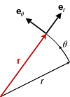
In two dimensions, the position vector , which has magnitude (length) and directed at an angle above the x-axis, can be expressed in Cartesian coordinates using the unit vectors and :[12]
The object moves with constant angular velocity around the circle. Therefore, where is time.
The velocity and acceleration of the motion are the first and second derivatives of position with respect to time:
The term in parentheses is the original expression of in Cartesian coordinates. Consequently,
negative shows that the acceleration is pointed towards the center of the circle (opposite the radius), hence it is called "centripetal" (i.e. "center-seeking"). While objects naturally follow a straight path (due to inertia), this centripetal acceleration describes the circular motion path caused by a centripetal force.
Derivation using vectors
Vector relationships for uniform circular motion; vector Ω representing the rotation is normal to the plane of the orbit with polarity determined by the right-hand rule and magnitude dθ /dt.
The image at right shows the vector relationships for uniform circular motion. The rotation itself is represented by the angular velocity vector Ω, which is normal to the plane of the orbit (using the right-hand rule) and has magnitude given by:
with θ the angular position at time t. In this subsection, dθ/dt is assumed constant, independent of time. The distance traveled dℓ of the particle in time dt along the circular path is
which, by properties of the vector cross product, has magnitude rdθ and is in the direction tangent to the circular path.
Applying Lagrange's formula with the observation that Ω • r(t) = 0 at all times,
In words, the acceleration is pointing directly opposite to the radial displacement r at all times, and has a magnitude:
where vertical bars |...| denote the vector magnitude, which in the case of r(t) is simply the radius r of the path. This result agrees with the previous section, though the notation is slightly different.
When the rate of rotation is made constant in the analysis of nonuniform circular motion, that analysis agrees with this one.
A merit of the vector approach is that it is manifestly independent of any coordinate system.
Upper panel: Ball on a banked circular track moving with constant speed v; Lower panel: Forces on the ball
The upper panel in the image at right shows a ball in circular motion on a banked curve. The curve is banked at an angle θ from the horizontal, and the surface of the road is considered to be slippery. The objective is to find what angle the bank must have so the ball does not slide off the road.[13] Intuition tells us that, on a flat curve with no banking at all, the ball will simply slide off the road; while with a very steep banking, the ball will slide to the center unless it travels the curve rapidly.
Apart from any acceleration that might occur in the direction of the path, the lower panel of the image above indicates the forces on the ball. There are two forces; one is the force of gravity vertically downward through the center of mass of the ball mg, where m is the mass of the ball and g is the gravitational acceleration; the second is the upward normal force exerted by the road at a right angle to the road surface man. The centripetal force demanded by the curved motion is also shown above. This centripetal force is not a third force applied to the ball, but rather must be provided by the net force on the ball resulting from vector addition of the normal force and the force of gravity. The resultant or net force on the ball found by vector addition of the normal force exerted by the road and vertical force due to gravity must equal the centripetal force dictated by the need to travel a circular path. The curved motion is maintained so long as this net force provides the centripetal force requisite to the motion.
The horizontal net force on the ball is the horizontal component of the force from the road, which has magnitude |Fh| = m|an| sin θ. The vertical component of the force from the road must counteract the gravitational force: |Fv| = m|an| cos θ = m|g|, which implies |an| = |g| / cos θ. Substituting into the above formula for |Fh| yields a horizontal force to be:
On the other hand, at velocity |v| on a circular path of radius r, kinematics says that the force needed to turn the ball continuously into the turn is the radially inward centripetal force Fc of magnitude:
Consequently, the ball is in a stable path when the angle of the road is set to satisfy the condition:
or,
As the angle of bank θ approaches 90°, the tangent function approaches infinity, allowing larger values for |v|2/r. In words, this equation states that for greater speeds (bigger |v|) the road must be banked more steeply (a larger value for θ), and for sharper turns (smaller r) the road also must be banked more steeply, which accords with intuition. When the angle θ does not satisfy the above condition, the horizontal component of force exerted by the road does not provide the correct centripetal force, and an additional frictional force tangential to the road surface is called upon to provide the difference. If friction cannot do this (that is, the coefficient of friction is exceeded), the ball slides to a different radius where the balance can be realized.[14][15]
These ideas apply to air flight as well. See the FAA pilot's manual.[16]
Velocity and acceleration for nonuniform circular motion: the velocity vector is tangential to the orbit, but the acceleration vector is not radially inward because of its tangential component aθ that increases the rate of rotation: dω / dt = |aθ| / R.
As a generalization of the uniform circular motion case, suppose the angular rate of rotation is not constant. The acceleration now has a tangential component, as shown the image at right. This case is used to demonstrate a derivation strategy based on a polar coordinate system.
Let r(t) be a vector that describes the position of a point mass as a function of time. Since we are assuming circular motion, let r(t) = R·ur, where R is a constant (the radius of the circle) and ur is the unit vector pointing from the origin to the point mass. The direction of ur is described by θ, the angle between the x-axis and the unit vector, measured counterclockwise from the x-axis. The other unit vector for polar coordinates, uθ is perpendicular to ur and points in the direction of increasing θ. These polar unit vectors can be expressed in terms of Cartesian unit vectors in the x and y directions, denoted and respectively:[17]
and
One can differentiate to find velocity:
where ω is the angular velocity dθ/dt.
This result for the velocity matches expectations that the velocity should be directed tangentially to the circle, and that the magnitude of the velocity should be rω. Differentiating again, and noting that
we find that the acceleration, a is:
Thus, the radial and tangential components of the acceleration are:
and
where |v| = rω is the magnitude of the velocity (the speed).
These equations express mathematically that, in the case of an object that moves along a circular path with a changing speed, the acceleration of the body may be decomposed into a perpendicular component that changes the direction of motion (the centripetal acceleration), and a parallel, or tangential component, that changes the speed.
Position vector r, always points radially from the origin.
Velocity vector v, always tangent to the path of motion.
Acceleration vector a, not parallel to the radial motion but offset by the angular and Coriolis accelerations, nor tangent to the path but offset by the centripetal and radial accelerations.
Kinematic vectors in plane polar coordinates. Notice the setup is not restricted to 2d space, but a plane in any higher dimension.
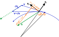
Polar unit vectors at two times t and t + dt for a particle with trajectory r ( t ); on the left the unit vectors uρ and uθ at the two times are moved so their tails all meet, and are shown to trace an arc of a unit radius circle. Their rotation in time dt is dθ, just the same angle as the rotation of the trajectory r ( t ).
Polar coordinates
The above results can be derived perhaps more simply in polar coordinates, and at the same time extended to general motion within a plane, as shown next. Polar coordinates in the plane employ a radial unit vector uρ and an angular unit vector uθ, as shown above.[18] A particle at position r is described by:
where the notation ρ is used to describe the distance of the path from the origin instead of R to emphasize that this distance is not fixed, but varies with time. The unit vector uρ travels with the particle and always points in the same direction as r(t). Unit vector uθ also travels with the particle and stays orthogonal to uρ. Thus, uρ and uθ form a local Cartesian coordinate system attached to the particle, and tied to the path travelled by the particle.[19] By moving the unit vectors so their tails coincide, as seen in the circle at the left of the image above, it is seen that uρ and uθ form a right-angled pair with tips on the unit circle that trace back and forth on the perimeter of this circle with the same angle θ(t) as r(t).
When the particle moves, its velocity is
To evaluate the velocity, the derivative of the unit vector uρ is needed. Because uρ is a unit vector, its magnitude is fixed, and it can change only in direction, that is, its change duρ has a component only perpendicular to uρ. When the trajectory r(t) rotates an amount dθ, uρ, which points in the same direction as r(t), also rotates by dθ. See image above. Therefore, the change in uρ is
or
In a similar fashion, the rate of change of uθ is found. As with uρ, uθ is a unit vector and can only rotate without changing size. To remain orthogonal to uρ while the trajectory r(t) rotates an amount dθ, uθ, which is orthogonal to r(t), also rotates by dθ. See image above. Therefore, the change duθ is orthogonal to uθ and proportional to dθ (see image above):
The equation above shows the sign to be negative: to maintain orthogonality, if duρ is positive with dθ, then duθ must decrease.
Substituting the derivative of uρ into the expression for velocity:
To obtain the acceleration, another time differentiation is done:
Substituting the derivatives of uρ and uθ, the acceleration of the particle is:[20]
As a particular example, if the particle moves in a circle of constant radius R, then dρ/dt = 0, v = vθ, and:
where
These results agree with those above for nonuniform circular motion. See also the article on non-uniform circular motion. If this acceleration is multiplied by the particle mass, the leading term is the centripetal force and the negative of the second term related to angular acceleration is sometimes called the Euler force.[21]
For trajectories other than circular motion, for example, the more general trajectory envisioned in the image above, the instantaneous center of rotation and radius of curvature of the trajectory are related only indirectly to the coordinate system defined by uρ and uθ and to the length |r(t)| = ρ. Consequently, in the general case, it is not straightforward to disentangle the centripetal and Euler terms from the above general acceleration equation.[22][23] To deal directly with this issue, local coordinates are preferable, as discussed next.
Local coordinates
Local coordinate system for planar motion on a curve. Two different positions are shown for distances s and s + ds along the curve. At each position s, unit vector un points along the outward normal to the curve and unit vector ut is tangential to the path. The radius of curvature of the path is ρ as found from the rate of rotation of the tangent to the curve with respect to arc length, and is the radius of the osculating circle at position s. The unit circle on the left shows the rotation of the unit vectors with s.
Local coordinates mean a set of coordinates that travel with the particle,[24] and have orientation determined by the path of the particle.[25] Unit vectors are formed as shown in the image at right, both tangential and normal to the path. This coordinate system sometimes is referred to as intrinsic or path coordinates[26][27] or nt-coordinates, for normal-tangential, referring to these unit vectors. These coordinates are a very special example of a more general concept of local coordinates from the theory of differential forms.[28]
Distance along the path of the particle is the arc length s, considered to be a known function of time.
A center of curvature is defined at each position s located a distance ρ (the radius of curvature) from the curve on a line along the normal un (s). The required distance ρ(s) at arc length s is defined in terms of the rate of rotation of the tangent to the curve, which in turn is determined by the path itself. If the orientation of the tangent relative to some starting position is θ(s), then ρ(s) is defined by the derivative dθ/ds:
The radius of curvature usually is taken as positive (that is, as an absolute value), while the curvatureκ is a signed quantity.
A geometric approach to finding the center of curvature and the radius of curvature uses a limiting process leading to the osculating circle.[29][30] See image above.
Using these coordinates, the motion along the path is viewed as a succession of circular paths of ever-changing center, and at each position s constitutes non-uniform circular motion at that position with radius ρ. The local value of the angular rate of rotation then is given by:
with the local speed v given by:
As for the other examples above, because unit vectors cannot change magnitude, their rate of change is always perpendicular to their direction (see the left-hand insert in the image above):[31]
Consequently, the velocity and acceleration are:[30][32][33]
In this local coordinate system, the acceleration resembles the expression for nonuniform circular motion with the local radius ρ(s), and the centripetal acceleration is identified as the second term.[34]
Looking at the image above, one might wonder whether adequate account has been taken of the difference in curvature between ρ(s) and ρ(s + ds) in computing the arc length as ds = ρ(s)dθ. Reassurance on this point can be found using a more formal approach outlined below. This approach also makes connection with the article on curvature.
To introduce the unit vectors of the local coordinate system, one approach is to begin in Cartesian coordinates and describe the local coordinates in terms of these Cartesian coordinates. In terms of arc length s, let the path be described as:[37]
Then an incremental displacement along the path ds is described by:
where primes are introduced to denote derivatives with respect to s. The magnitude of this displacement is ds, showing that:[38]
(Eq. 1)
This displacement is necessarily a tangent to the curve at s, showing that the unit vector tangent to the curve is:
while the outward unit vector normal to the curve is
Orthogonality can be verified by showing that the vector dot product is zero. The unit magnitude of these vectors is a consequence of Eq. 1. Using the tangent vector, the angle θ of the tangent to the curve is given by:
and
The radius of curvature is introduced completely formally (without need for geometric interpretation) as:
The derivative of θ can be found from that for sinθ:
Now:
in which the denominator is unity. With this formula for the derivative of the sine, the radius of curvature becomes:
where the equivalence of the forms stems from differentiation of Eq. 1:
With these results, the acceleration can be found:
as can be verified by taking the dot product with the unit vectors ut(s) and un(s). This result for acceleration is the same as that for circular motion based on the radius ρ. Using this coordinate system in the inertial frame, it is easy to identify the force normal to the trajectory as the centripetal force and that parallel to the trajectory as the tangential force. From a qualitative standpoint, the path can be approximated by an arc of a circle for a limited time, and for the limited time a particular radius of curvature applies, the centrifugal and Euler forces can be analyzed on the basis of circular motion with that radius.
This result for acceleration agrees with that found earlier. However, in this approach, the question of the change in radius of curvature with s is handled completely formally, consistent with a geometric interpretation, but not relying upon it, thereby avoiding any questions the image above might suggest about neglecting the variation in ρ.
Example: circular motion
To illustrate the above formulas, let x, y be given as:
Then:
which can be recognized as a circular path around the origin with radius α. The position s = 0 corresponds to [α, 0], or 3 o'clock. To use the above formalism, the derivatives are needed:
With these results, one can verify that:
The unit vectors can also be found:
which serve to show that s = 0 is located at position [ρ, 0] and s = ρπ/2 at [0, ρ], which agrees with the original expressions for x and y. In other words, s is measured counterclockwise around the circle from 3 o'clock. Also, the derivatives of these vectors can be found:
To obtain velocity and acceleration, a time-dependence for s is necessary. For counterclockwise motion at variable speed v(t):
where v(t) is the speed and t is time, and s(t = 0) = 0. Then:
where it already is established that α = ρ. This acceleration is the standard result for non-uniform circular motion.
↑ Chris Carter (2001). Facts and Practice for A-Level: Physics. S.2.: Oxford University Press. p.30. ISBN978-0-19-914768-7.{{cite book}}: CS1 maint: location (link)
↑ Note: unlike the Cartesian unit vectors and , which are constant, in polar coordinates the direction of the unit vectors ur and uθ depend on θ, and so in general have non-zero time derivatives.
↑ Although the polar coordinate system moves with the particle, the observer does not. The description of the particle motion remains a description from the stationary observer's point of view.
↑ Notice that this local coordinate system is not autonomous; for example, its rotation in time is dictated by the trajectory traced by the particle. The radial vector r(t) does not represent the radius of curvature of the path.
↑ The observer of the motion along the curve is using these local coordinates to describe the motion from the observer's frame of reference, that is, from a stationary point of view. In other words, although the local coordinate system moves with the particle, the observer does not. A change in coordinate system used by the observer is only a change in their description of observations, and does not mean that the observer has changed their state of motion, and vice versa.
↑ The osculating circle at a given point P on a curve is the limiting circle of a sequence of circles that pass through P and two other points on the curve, Q and R, on either side of P, as Q and R approach P. See the online text by Lamb: Horace Lamb (1897). An Elementary Course of Infinitesimal Calculus. University Press. p.406. ISBN978-1-108-00534-0. osculating circle.
↑ The article on curvature treats a more general case where the curve is parametrized by an arbitrary variable (denoted t), rather than by the arc length s.
Tipler, Paul (2004). Physics for Scientists and Engineers: Mechanics, Oscillations and Waves, Thermodynamics (5thed.). W. H. Freeman. ISBN978-0-7167-0809-4.
In mathematics, a spherical coordinate system is a coordinate system for three-dimensional space where the position of a given point in space is specified by three numbers, : the radial distance of the radial liner connecting the point to the fixed point of origin ; the polar angle θ of the radial line r; and the azimuthal angle φ of the radial line r.
The Navier–Stokes equations are partial differential equations which describe the motion of viscous fluid substances. They were named after French engineer and physicist Claude-Louis Navier and the Irish physicist and mathematician George Gabriel Stokes. They were developed over several decades of progressively building the theories, from 1822 (Navier) to 1842–1850 (Stokes).
Kinematics is a subfield of physics, developed in classical mechanics, that describes the motion of points, bodies (objects), and systems of bodies without considering the forces that cause them to move. Kinematics, as a field of study, is often referred to as the "geometry of motion" and is occasionally seen as a branch of mathematics. A kinematics problem begins by describing the geometry of the system and declaring the initial conditions of any known values of position, velocity and/or acceleration of points within the system. Then, using arguments from geometry, the position, velocity and acceleration of any unknown parts of the system can be determined. The study of how forces act on bodies falls within kinetics, not kinematics. For further details, see analytical dynamics.
In mathematics, a unit vector in a normed vector space is a vector of length 1. A unit vector is often denoted by a lowercase letter with a circumflex, or "hat", as in .
In mathematics, the Laplace operator or Laplacian is a differential operator given by the divergence of the gradient of a scalar function on Euclidean space. It is usually denoted by the symbols , (where is the nabla operator), or . In a Cartesian coordinate system, the Laplacian is given by the sum of second partial derivatives of the function with respect to each independent variable. In other coordinate systems, such as cylindrical and spherical coordinates, the Laplacian also has a useful form. Informally, the Laplacian Δf (p) of a function f at a point p measures by how much the average value of f over small spheres or balls centered at p deviates from f (p).
In fluid dynamics, Stokes' law is an empirical law for the frictional force – also called drag force – exerted on spherical objects with very small Reynolds numbers in a viscous fluid. It was derived by George Gabriel Stokes in 1851 by solving the Stokes flow limit for small Reynolds numbers of the Navier–Stokes equations.
In physics, circular motion is a movement of an object along the circumference of a circle or rotation along a circular arc. It can be uniform, with a constant rate of rotation and constant tangential speed, or non-uniform with a changing rate of rotation. The rotation around a fixed axis of a three-dimensional body involves the circular motion of its parts. The equations of motion describe the movement of the center of mass of a body, which remains at a constant distance from the axis of rotation. In circular motion, the distance between the body and a fixed point on its surface remains the same, i.e., the body is assumed rigid.
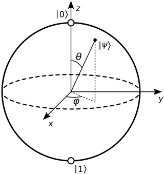
In quantum mechanics and computing, the Bloch sphere is a geometrical representation of the pure state space of a two-level quantum mechanical system (qubit), named after the physicist Felix Bloch.
This is a list of some vector calculus formulae for working with common curvilinear coordinate systems.
Note: This page uses common physics notation for spherical coordinates, in which is the angle between the z axis and the radius vector connecting the origin to the point in question, while is the angle between the projection of the radius vector onto the x-y plane and the x axis. Several other definitions are in use, and so care must be taken in comparing different sources.
In physics, the Hamilton–Jacobi equation, named after William Rowan Hamilton and Carl Gustav Jacob Jacobi, is an alternative formulation of classical mechanics, equivalent to other formulations such as Newton's laws of motion, Lagrangian mechanics and Hamiltonian mechanics.
A fictitious force is a force that appears to act on a mass whose motion is described using a non-inertial frame of reference, such as a linearly accelerating or rotating reference frame. It is related to Newton's second law of motion, which treats forces for just one object.
A rotating frame of reference is a special case of a non-inertial reference frame that is rotating relative to an inertial reference frame. An everyday example of a rotating reference frame is the surface of the Earth.
Euler–Bernoulli beam theory is a simplification of the linear theory of elasticity which provides a means of calculating the load-carrying and deflection characteristics of beams. It covers the case corresponding to small deflections of a beam that is subjected to lateral loads only. By ignoring the effects of shear deformation and rotatory inertia, it is thus a special case of Timoshenko–Ehrenfest beam theory. It was first enunciated circa 1750, but was not applied on a large scale until the development of the Eiffel Tower and the Ferris wheel in the late 19th century. Following these successful demonstrations, it quickly became a cornerstone of engineering and an enabler of the Second Industrial Revolution.
In mathematics, vector spherical harmonics (VSH) are an extension of the scalar spherical harmonics for use with vector fields. The components of the VSH are complex-valued functions expressed in the spherical coordinate basis vectors.
In fluid dynamics, the Oseen equations describe the flow of a viscous and incompressible fluid at small Reynolds numbers, as formulated by Carl Wilhelm Oseen in 1910. Oseen flow is an improved description of these flows, as compared to Stokes flow, with the (partial) inclusion of convective acceleration.
Mechanics of planar particle motion is the analysis of the motion of particles gravitationally attracted to one another observed from non-inertial reference frames and the generalization of this problem to planetary motion. This type of analysis is closely related to centrifugal force, two-body problem, orbit and Kepler's laws of planetary motion. The mechanics of planar particle motion fall in the general field of analytical dynamics, and helps determining orbits from the given force laws. This article is focused more on the kinematic issues surrounding planar motion, which are the determination of the forces necessary to result in a certain trajectory given the particle trajectory.
In mathematics, potential flow around a circular cylinder is a classical solution for the flow of an inviscid, incompressible fluid around a cylinder that is transverse to the flow. Far from the cylinder, the flow is unidirectional and uniform. The flow has no vorticity and thus the velocity field is irrotational and can be modeled as a potential flow. Unlike a real fluid, this solution indicates a net zero drag on the body, a result known as d'Alembert's paradox.
In optics, the Fraunhofer diffraction equation is used to model the diffraction of waves when the diffraction pattern is viewed at a long distance from the diffracting object, and also when it is viewed at the focal plane of an imaging lens.
Blade element momentum theory is a theory that combines both blade element theory and momentum theory. It is used to calculate the local forces on a propeller or wind-turbine blade. Blade element theory is combined with momentum theory to alleviate some of the difficulties in calculating the induced velocities at the rotor.
This page is based on this Wikipedia article Text is available under the CC BY-SA 4.0 license; additional terms may apply. Images, videos and audio are available under their respective licenses.