Cosine similarity

Last updated

In data analysis, cosine similarity is a measure of similarity between two non-zero vectors defined in an inner product space. Cosine similarity is the cosine of the angle between the vectors; that is, it is the dot product of the vectors divided by the product of their lengths. It follows that the cosine similarity does not depend on the magnitudes of the vectors, but only on their angle. The cosine similarity always belongs to the interval For example, two proportional vectors have a cosine similarity of 1, two orthogonal vectors have a similarity of 0, and two opposite vectors have a similarity of -1. In some contexts, the component values of the vectors cannot be negative, in which case the cosine similarity is bounded in .

Contents

For example, in information retrieval and text mining, each word is assigned a different coordinate and a document is represented by the vector of the numbers of occurrences of each word in the document. Cosine similarity then gives a useful measure of how similar two documents are likely to be, in terms of their subject matter, and independently of the length of the documents. [1]

The technique is also used to measure cohesion within clusters in the field of data mining. [2]

One advantage of cosine similarity is its low complexity, especially for sparse vectors: only the non-zero coordinates need to be considered.

Other names for cosine similarity include Orchini similarity and Tucker coefficient of congruence; the Otsuka–Ochiai similarity (see below) is cosine similarity applied to binary data.

Definition

The cosine of two non-zero vectors can be derived by using the Euclidean dot product formula:

Given two n-dimensional vectors of attributes, A and B, the cosine similarity, cos(θ), is represented using a dot product and magnitude as

where and are the th components of vectors and , respectively.

The resulting similarity ranges from -1 meaning exactly opposite, to 1 meaning exactly the same, with 0 indicating orthogonality or decorrelation, while in-between values indicate intermediate similarity or dissimilarity.

For text matching, the attribute vectors A and B are usually the term frequency vectors of the documents. Cosine similarity can be seen as a method of normalizing document length during comparison. In the case of information retrieval, the cosine similarity of two documents will range from , since the term frequencies cannot be negative. This remains true when using TF-IDF weights. The angle between two term frequency vectors cannot be greater than 90°.

If the attribute vectors are normalized by subtracting the vector means (e.g., ), the measure is called the centered cosine similarity and is equivalent to the Pearson correlation coefficient. For an example of centering,

Cosine distance

The term cosine distance [3] is commonly used for the complement of cosine similarity in positive space, that is

It is important to note that the cosine distance is not a true distance metric as it does not exhibit the triangle inequality property—or, more formally, the Schwarz inequality—and it violates the coincidence axiom. One way to see this is to note that the cosine distance is half of the squared Euclidean distance of the normalization of the vectors, and squared Euclidean distance does not satisfy the triangle inequality either. To repair the triangle inequality property while maintaining the same ordering, it is necessary to convert to angular distance or Euclidean distance. Alternatively, the triangular inequality that does work for angular distances can be expressed directly in terms of the cosines; see below.

Angular distance and similarity

The normalized angle, referred to as angular distance, between any two vectors and is a formal distance metric and can be calculated from the cosine similarity. [4] The complement of the angular distance metric can then be used to define angular similarity function bounded between 0 and 1, inclusive.

When the vector elements may be positive or negative:

Or, if the vector elements are always positive:

Unfortunately, computing the inverse cosine (arccos) function is slow, making the use of the angular distance more computationally expensive than using the more common (but not metric) cosine distance above.

L2-normalized Euclidean distance

Another effective proxy for cosine distance can be obtained by normalisation of the vectors, followed by the application of normal Euclidean distance. Using this technique each term in each vector is first divided by the magnitude of the vector, yielding a vector of unit length. Then the Euclidean distance over the end-points of any two vectors is a proper metric which gives the same ordering as the cosine distance (a monotonic transformation of Euclidean distance; see below) for any comparison of vectors, and furthermore avoids the potentially expensive trigonometric operations required to yield a proper metric. Once the normalisation has occurred, the vector space can be used with the full range of techniques available to any Euclidean space, notably standard dimensionality reduction techniques. This normalised form distance is often used within many deep learning algorithms.

Otsuka–Ochiai coefficient

In biology, there is a similar concept known as the Otsuka–Ochiai coefficient named after Yanosuke Otsuka (also spelled as Ōtsuka, Ootsuka or Otuka, [5] Japanese : 大塚 弥之助) [6] and Akira Ochiai (Japanese : 落合 明), [7] also known as the Ochiai–Barkman [8] or Ochiai coefficient, [9] which can be represented as:

Here, and are sets, and is the number of elements in . If sets are represented as bit vectors, the Otsuka–Ochiai coefficient can be seen to be the same as the cosine similarity. It is identical to the score introduced by Godfrey Thomson. [10]

In a recent book, [11] the coefficient is tentatively misattributed to another Japanese researcher with the family name Otsuka. The confusion arises because in 1957 Akira Ochiai attributes the coefficient only to Otsuka (no first name mentioned) [7] by citing an article by Ikuso Hamai (Japanese : 浜井 生三), [12] who in turn cites the original 1936 article by Yanosuke Otsuka. [6]

Properties

The most noteworthy property of cosine similarity is that it reflects a relative, rather than absolute, comparison of the individual vector dimensions. For any constant and vector , the vectors and are maximally similar. The measure is thus most appropriate for data where frequency is more important than absolute values; notably, term frequency in documents. However more recent metrics with a grounding in information theory, such as Jensen–Shannon, SED, and triangular divergence have been shown to have improved semantics in at least some contexts. [13]

Cosine similarity is related to Euclidean distance as follows. Denote Euclidean distance by the usual , and observe that

(polarization identity)

by expansion. When A and B are normalized to unit length, so this expression is equal to

In short, the cosine distance can be expressed in terms of Euclidean distance as

.

The Euclidean distance is called the chord distance (because it is the length of the chord on the unit circle) and it is the Euclidean distance between the vectors which were normalized to unit sum of squared values within them.

Null distribution: For data which can be negative as well as positive, the null distribution for cosine similarity is the distribution of the dot product of two independent random unit vectors. This distribution has a mean of zero and a variance of (where is the number of dimensions), and although the distribution is bounded between -1 and +1, as grows large the distribution is increasingly well-approximated by the normal distribution. [14] [15] Other types of data such as bitstreams, which only take the values 0 or 1, the null distribution takes a different form and may have a nonzero mean. [16]

Triangle inequality for cosine similarity

The ordinary triangle inequality for angles (i.e., arc lengths on a unit hypersphere) gives us that

Because the cosine function decreases as an angle in [0, π] radians increases, the sense of these inequalities is reversed when we take the cosine of each value:

Using the cosine addition and subtraction formulas, these two inequalities can be written in terms of the original cosines,

This form of the triangle inequality can be used to bound the minimum and maximum similarity of two objects A and B if the similarities to a reference object C is already known. This is used for example in metric data indexing, but has also been used to accelerate spherical k-means clustering [17] the same way the Euclidean triangle inequality has been used to accelerate regular k-means.

Soft cosine measure

A soft cosine or ("soft" similarity) between two vectors considers similarities between pairs of features. [18] The traditional cosine similarity considers the vector space model (VSM) features as independent or completely different, while the soft cosine measure proposes considering the similarity of features in VSM, which help generalize the concept of cosine (and soft cosine) as well as the idea of (soft) similarity.

For example, in the field of natural language processing (NLP) the similarity among features is quite intuitive. Features such as words, n-grams, or syntactic n-grams [19] can be quite similar, though formally they are considered as different features in the VSM. For example, words “play” and “game” are different words and thus mapped to different points in VSM; yet they are semantically related. In case of n-grams or syntactic n-grams, Levenshtein distance can be applied (in fact, Levenshtein distance can be applied to words as well).

For calculating soft cosine, the matrix s is used to indicate similarity between features. It can be calculated through Levenshtein distance, WordNet similarity, or other similarity measures. Then we just multiply by this matrix.

Given two N-dimension vectors and , the soft cosine similarity is calculated as follows:

where sij = similarity(featurei, featurej).

If there is no similarity between features (sii = 1, sij = 0 for ij), the given equation is equivalent to the conventional cosine similarity formula.

The time complexity of this measure is quadratic, which makes it applicable to real-world tasks. Note that the complexity can be reduced to subquadratic. [20] An efficient implementation of such soft cosine similarity is included in the Gensim open source library.

See also

Related Research Articles

Kinematics is a subfield of physics and mathematics, developed in classical mechanics, that describes the motion of points, bodies (objects), and systems of bodies without considering the forces that cause them to move. Kinematics, as a field of study, is often referred to as the "geometry of motion" and is occasionally seen as a branch of both applied and pure mathematics since it can be studied without considering the mass of a body or the forces acting upon it. A kinematics problem begins by describing the geometry of the system and declaring the initial conditions of any known values of position, velocity and/or acceleration of points within the system. Then, using arguments from geometry, the position, velocity and acceleration of any unknown parts of the system can be determined. The study of how forces act on bodies falls within kinetics, not kinematics. For further details, see analytical dynamics.

In mathematics, the dot product or scalar product is an algebraic operation that takes two equal-length sequences of numbers, and returns a single number. In Euclidean geometry, the dot product of the Cartesian coordinates of two vectors is widely used. It is often called the inner product of Euclidean space, even though it is not the only inner product that can be defined on Euclidean space.

<span class="mw-page-title-main">Unit vector</span> Vector of length one

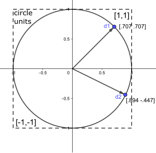
In mathematics, a unit vector in a normed vector space is a vector of length 1. A unit vector is often denoted by a lowercase letter with a circumflex, or "hat", as in .

In mechanics and geometry, the 3D rotation group, often denoted SO(3), is the group of all rotations about the origin of three-dimensional Euclidean space under the operation of composition.

In mathematics, the Laplace operator or Laplacian is a differential operator given by the divergence of the gradient of a scalar function on Euclidean space. It is usually denoted by the symbols , (where is the nabla operator), or . In a Cartesian coordinate system, the Laplacian is given by the sum of second partial derivatives of the function with respect to each independent variable. In other coordinate systems, such as cylindrical and spherical coordinates, the Laplacian also has a useful form. Informally, the Laplacian Δf (p) of a function f at a point p measures by how much the average value of f over small spheres or balls centered at p deviates from f (p).

Unit quaternions, known as versors, provide a convenient mathematical notation for representing spatial orientations and rotations of elements in three dimensional space. Specifically, they encode information about an axis-angle rotation about an arbitrary axis. Rotation and orientation quaternions have applications in computer graphics, computer vision, robotics, navigation, molecular dynamics, flight dynamics, orbital mechanics of satellites, and crystallographic texture analysis.

In the mathematical field of differential geometry, a metric tensor is an additional structure on a manifold M that allows defining distances and angles, just as the inner product on a Euclidean space allows defining distances and angles there. More precisely, a metric tensor at a point p of M is a bilinear form defined on the tangent space at p, and a metric field on M consists of a metric tensor at each point p of M that varies smoothly with p.

<span class="mw-page-title-main">Spherical harmonics</span> Special mathematical functions defined on the surface of a sphere

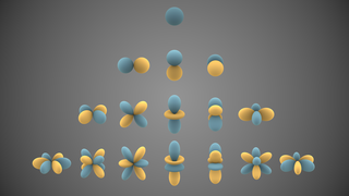
In mathematics and physical science, spherical harmonics are special functions defined on the surface of a sphere. They are often employed in solving partial differential equations in many scientific fields. The table of spherical harmonics contains a list of common spherical harmonics.

In linear algebra, linear transformations can be represented by matrices. If is a linear transformation mapping to and is a column vector with entries, then

In mathematics and physics, the Christoffel symbols are an array of numbers describing a metric connection. The metric connection is a specialization of the affine connection to surfaces or other manifolds endowed with a metric, allowing distances to be measured on that surface. In differential geometry, an affine connection can be defined without reference to a metric, and many additional concepts follow: parallel transport, covariant derivatives, geodesics, etc. also do not require the concept of a metric. However, when a metric is available, these concepts can be directly tied to the "shape" of the manifold itself; that shape is determined by how the tangent space is attached to the cotangent space by the metric tensor. Abstractly, one would say that the manifold has an associated (orthonormal) frame bundle, with each "frame" being a possible choice of a coordinate frame. An invariant metric implies that the structure group of the frame bundle is the orthogonal group O(p, q). As a result, such a manifold is necessarily a (pseudo-)Riemannian manifold. The Christoffel symbols provide a concrete representation of the connection of (pseudo-)Riemannian geometry in terms of coordinates on the manifold. Additional concepts, such as parallel transport, geodesics, etc. can then be expressed in terms of Christoffel symbols.

<span class="mw-page-title-main">Vector projection</span> Concept in linear algebra

The vector projection of a vector a on a nonzero vector b is the orthogonal projection of a onto a straight line parallel to b. The projection of a onto b is often written as or ab.

A parametric surface is a surface in the Euclidean space which is defined by a parametric equation with two parameters . Parametric representation is a very general way to specify a surface, as well as implicit representation. Surfaces that occur in two of the main theorems of vector calculus, Stokes' theorem and the divergence theorem, are frequently given in a parametric form. The curvature and arc length of curves on the surface, surface area, differential geometric invariants such as the first and second fundamental forms, Gaussian, mean, and principal curvatures can all be computed from a given parametrization.

Angular distance or angular separation is the measure of the angle between the orientation of two straight lines, rays, or vectors in three-dimensional space, or the central angle subtended by the radii through two points on a sphere. When the rays are lines of sight from an observer to two points in space, it is known as the apparent distance or apparent separation.

In geometry, various formalisms exist to express a rotation in three dimensions as a mathematical transformation. In physics, this concept is applied to classical mechanics where rotational kinematics is the science of quantitative description of a purely rotational motion. The orientation of an object at a given instant is described with the same tools, as it is defined as an imaginary rotation from a reference placement in space, rather than an actually observed rotation from a previous placement in space.

<span class="mw-page-title-main">Axis–angle representation</span> Parameterization of a rotation into a unit vector and angle

In mathematics, the axis–angle representation parameterizes a rotation in a three-dimensional Euclidean space by two quantities: a unit vector e indicating the direction (geometry) of an axis of rotation, and an angle of rotation θ describing the magnitude and sense of the rotation about the axis. Only two numbers, not three, are needed to define the direction of a unit vector e rooted at the origin because the magnitude of e is constrained. For example, the elevation and azimuth angles of e suffice to locate it in any particular Cartesian coordinate frame.

In mathematics and statistics, a circular mean or angular mean is a mean designed for angles and similar cyclic quantities, such as times of day, and fractional parts of real numbers.

<span class="mw-page-title-main">Kepler orbit</span> Celestial orbit whose trajectory is a conic section in the orbital plane

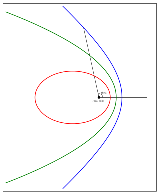
In celestial mechanics, a Kepler orbit is the motion of one body relative to another, as an ellipse, parabola, or hyperbola, which forms a two-dimensional orbital plane in three-dimensional space. A Kepler orbit can also form a straight line. It considers only the point-like gravitational attraction of two bodies, neglecting perturbations due to gravitational interactions with other objects, atmospheric drag, solar radiation pressure, a non-spherical central body, and so on. It is thus said to be a solution of a special case of the two-body problem, known as the Kepler problem. As a theory in classical mechanics, it also does not take into account the effects of general relativity. Keplerian orbits can be parametrized into six orbital elements in various ways.

<span class="mw-page-title-main">Pythagorean theorem</span> Relation between sides of a right triangle

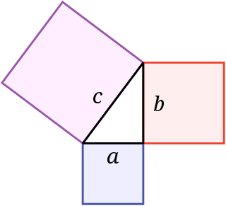
In mathematics, the Pythagorean theorem or Pythagoras' theorem is a fundamental relation in Euclidean geometry between the three sides of a right triangle. It states that the area of the square whose side is the hypotenuse is equal to the sum of the areas of the squares on the other two sides.

The following are important identities in vector algebra. Identities that involve the magnitude of a vector , or the dot product of two vectors A·B, apply to vectors in any dimension. Identities that use the cross product A×B are defined only in three dimensions. Most of these relations can be dated to founder of vector calculus Josiah Willard Gibbs, if not earlier.

In orbital mechanics, Gauss's method is used for preliminary orbit determination from at least three observations of the orbiting body of interest at three different times. The required information are the times of observations, the position vectors of the observation points, the direction cosine vector of the orbiting body from the observation points and general physical data.

References

  1. Singhal, Amit (2001). "Modern Information Retrieval: A Brief Overview". Bulletin of the IEEE Computer Society Technical Committee on Data Engineering 24 (4): 35–43.
  2. P.-N. Tan, M. Steinbach & V. Kumar, Introduction to Data Mining, Addison-Wesley (2005), ISBN   0-321-32136-7, chapter 8; page 500.
  3. Wolfram Research (2007). "CosineDistance – Wolfram Language & System Documentation Center". wolfram.com.{{cite web}}: CS1 maint: numeric names: authors list (link)
  4. "COSINE DISTANCE, COSINE SIMILARITY, ANGULAR COSINE DISTANCE, ANGULAR COSINE SIMILARITY". www.itl.nist.gov. Retrieved 2020-07-11.
  5. Omori, Masae (2004). "Geological idea of Yanosuke Otuka, who built the foundation of neotectonics (geoscientist)". Earth Science. 58 (4): 256–259. doi:10.15080/agcjchikyukagaku.58.4_256.
  6. 1 2 Otsuka, Yanosuke (1936). "The faunal character of the Japanese Pleistocene marine Mollusca, as evidence of the climate having become colder during the Pleistocene in Japan". Bulletin of the Biogeographical Society of Japan. 6 (16): 165–170.
  7. 1 2 Ochiai, Akira (1957). "Zoogeographical studies on the soleoid fishes found in Japan and its neighhouring regions-II". Bulletin of the Japanese Society of Scientific Fisheries. 22 (9): 526–530. doi: 10.2331/suisan.22.526 .
  8. Barkman, Jan J. (1958). Phytosociology and Ecology of Cryptogamic Epiphytes: Including a Taxonomic Survey and Description of Their Vegetation Units in Europe. Assen: Van Gorcum.
  9. Romesburg, H. Charles (1984). Cluster Analysis for Researchers. Belmont, California: Lifetime Learning Publications. p. 149.
  10. Thomson, Godfrey (1916). "A hierarchy without a general factor" (PDF). British Journal of Psychology. 8: 271–281.
  11. Howarth, Richard J. (2017). Dictionary of Mathematical Geosciences: With Historical Notes. Cham: Springer. p. 421. doi:10.1007/978-3-319-57315-1. ISBN   978-3-319-57314-4. S2CID   67081034. […] attributed by him to "Otsuka" [?A. Otsuka of the Dept. of Fisheries, Tohoku University].
  12. Hamai, Ikuso (1955). "Stratification of community by means of "community coefficient" (continued)". Japanese Journal of Ecology. 5 (1): 41–45. doi:10.18960/seitai.5.1_41.
  13. Connor, Richard (2016). A Tale of Four Metrics. Similarity Search and Applications. Tokyo: Springer. doi:10.1007/978-3-319-46759-7_16.
  14. Spruill, Marcus C. (2007). "Asymptotic distribution of coordinates on high dimensional spheres". Electronic Communications in Probability. 12: 234–247. doi: 10.1214/ECP.v12-1294 .
  15. "Distribution of dot products between two random unit vectors in RD". CrossValidated.
  16. Graham L. Giller (2012). "The Statistical Properties of Random Bitstreams and the Sampling Distribution of Cosine Similarity". Giller Investments Research Notes (20121024/1). doi:10.2139/ssrn.2167044. S2CID   123332455.
  17. Schubert, Erich; Lang, Andreas; Feher, Gloria (2021). Reyes, Nora; Connor, Richard; Kriege, Nils; Kazempour, Daniyal; Bartolini, Ilaria; Schubert, Erich; Chen, Jian-Jia (eds.). "Accelerating Spherical k-Means". Similarity Search and Applications. Lecture Notes in Computer Science. 13058. Cham: Springer International Publishing: 217–231. arXiv: 2107.04074 . doi:10.1007/978-3-030-89657-7_17. ISBN   978-3-030-89657-7. S2CID   235790358.
  18. Sidorov, Grigori; Gelbukh, Alexander; Gómez-Adorno, Helena; Pinto, David (29 September 2014). "Soft Similarity and Soft Cosine Measure: Similarity of Features in Vector Space Model". Computación y Sistemas. 18 (3): 491–504. doi:10.13053/CyS-18-3-2043 . Retrieved 7 October 2014.
  19. Sidorov, Grigori; Velasquez, Francisco; Stamatatos, Efstathios; Gelbukh, Alexander; Chanona-Hernández, Liliana (2013). Advances in Computational Intelligence. Lecture Notes in Computer Science. Vol. 7630. LNAI 7630. pp. 1–11. doi:10.1007/978-3-642-37798-3_1. ISBN   978-3-642-37798-3.
  20. Novotný, Vít (2018). Implementation Notes for the Soft Cosine Measure. The 27th ACM International Conference on Information and Knowledge Management. Torun, Italy: Association for Computing Machinery. pp. 1639–1642. arXiv: 1808.09407 . doi:10.1145/3269206.3269317. ISBN   978-1-4503-6014-2.