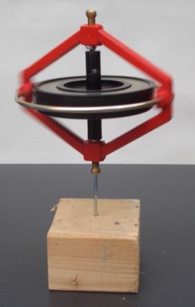
In physics, angular momentum is the rotational analog of linear momentum. It is an important physical quantity because it is a conserved quantity – the total angular momentum of a closed system remains constant. Angular momentum has both a direction and a magnitude, and both are conserved. Bicycles and motorcycles, flying discs, rifled bullets, and gyroscopes owe their useful properties to conservation of angular momentum. Conservation of angular momentum is also why hurricanes form spirals and neutron stars have high rotational rates. In general, conservation limits the possible motion of a system, but it does not uniquely determine it.
In classical mechanics, a harmonic oscillator is a system that, when displaced from its equilibrium position, experiences a restoring force F proportional to the displacement x:

The Navier–Stokes equations are partial differential equations which describe the motion of viscous fluid substances. They were named after French engineer and physicist Claude-Louis Navier and the Irish physicist and mathematician George Gabriel Stokes. They were developed over several decades of progressively building the theories, from 1822 (Navier) to 1842–1850 (Stokes).
In physics, equations of motion are equations that describe the behavior of a physical system in terms of its motion as a function of time. More specifically, the equations of motion describe the behavior of a physical system as a set of mathematical functions in terms of dynamic variables. These variables are usually spatial coordinates and time, but may include momentum components. The most general choice are generalized coordinates which can be any convenient variables characteristic of the physical system. The functions are defined in a Euclidean space in classical mechanics, but are replaced by curved spaces in relativity. If the dynamics of a system is known, the equations are the solutions for the differential equations describing the motion of the dynamics.
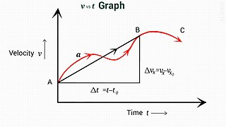
Kinematics is a subfield of physics, developed in classical mechanics, that describes the motion of points, bodies (objects), and systems of bodies without considering the forces that cause them to move. Kinematics, as a field of study, is often referred to as the "geometry of motion" and is occasionally seen as a branch of mathematics. A kinematics problem begins by describing the geometry of the system and declaring the initial conditions of any known values of position, velocity and/or acceleration of points within the system. Then, using arguments from geometry, the position, velocity and acceleration of any unknown parts of the system can be determined. The study of how forces act on bodies falls within kinetics, not kinematics. For further details, see analytical dynamics.

In physics, angular velocity, also known as angular frequency vector, is a pseudovector representation of how the angular position or orientation of an object changes with time, i.e. how quickly an object rotates around an axis of rotation and how fast the axis itself changes direction.
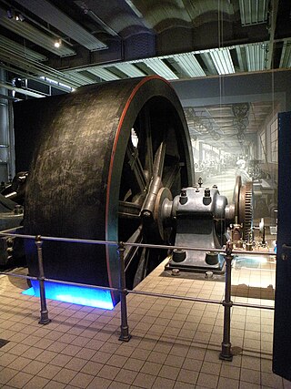
The moment of inertia, otherwise known as the mass moment of inertia, angular mass, second moment of mass, or most accurately, rotational inertia, of a rigid body is a quantity that determines the torque needed for a desired angular acceleration about a rotational axis, akin to how mass determines the force needed for a desired acceleration. It depends on the body's mass distribution and the axis chosen, with larger moments requiring more torque to change the body's rate of rotation by a given amount.
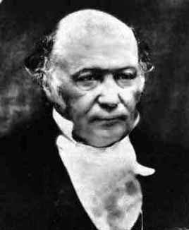
Hamiltonian mechanics emerged in 1833 as a reformulation of Lagrangian mechanics. Introduced by Sir William Rowan Hamilton, Hamiltonian mechanics replaces (generalized) velocities used in Lagrangian mechanics with (generalized) momenta. Both theories provide interpretations of classical mechanics and describe the same physical phenomena.
In mathematics, a linear form is a linear map from a vector space to its field of scalars.
In mathematics, the Hodge star operator or Hodge star is a linear map defined on the exterior algebra of a finite-dimensional oriented vector space endowed with a nondegenerate symmetric bilinear form. Applying the operator to an element of the algebra produces the Hodge dual of the element. This map was introduced by W. V. D. Hodge.
An infinitesimal rotation matrix or differential rotation matrix is a matrix representing an infinitely small rotation.
In rotordynamics, the rigid rotor is a mechanical model of rotating systems. An arbitrary rigid rotor is a 3-dimensional rigid object, such as a top. To orient such an object in space requires three angles, known as Euler angles. A special rigid rotor is the linear rotor requiring only two angles to describe, for example of a diatomic molecule. More general molecules are 3-dimensional, such as water, ammonia, or methane.
Screw theory is the algebraic calculation of pairs of vectors, such as angular and linear velocity, or forces and moments, that arise in the kinematics and dynamics of rigid bodies.
In calculus, the Leibniz integral rule for differentiation under the integral sign states that for an integral of the form
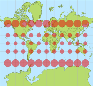
In cartography, a Tissot's indicatrix is a mathematical contrivance presented by French mathematician Nicolas Auguste Tissot in 1859 and 1871 in order to characterize local distortions due to map projection. It is the geometry that results from projecting a circle of infinitesimal radius from a curved geometric model, such as a globe, onto a map. Tissot proved that the resulting diagram is an ellipse whose axes indicate the two principal directions along which scale is maximal and minimal at that point on the map.

In mathematics, the Weierstrass–Enneper parameterization of minimal surfaces is a classical piece of differential geometry.
The angular velocity tensor is a skew-symmetric matrix defined by:
In general relativity, Lense–Thirring precession or the Lense–Thirring effect is a relativistic correction to the precession of a gyroscope near a large rotating mass such as the Earth. It is a gravitomagnetic frame-dragging effect. It is a prediction of general relativity consisting of secular precessions of the longitude of the ascending node and the argument of pericenter of a test particle freely orbiting a central spinning mass endowed with angular momentum .
In mathematics, vector spherical harmonics (VSH) are an extension of the scalar spherical harmonics for use with vector fields. The components of the VSH are complex-valued functions expressed in the spherical coordinate basis vectors.

In fluid dynamics, the mild-slope equation describes the combined effects of diffraction and refraction for water waves propagating over bathymetry and due to lateral boundaries—like breakwaters and coastlines. It is an approximate model, deriving its name from being originally developed for wave propagation over mild slopes of the sea floor. The mild-slope equation is often used in coastal engineering to compute the wave-field changes near harbours and coasts.


