Earnshaw's theorem

Last updated

Earnshaw's theorem states that a collection of point charges cannot be maintained in a stable stationary equilibrium configuration solely by the electrostatic interaction of the charges. This was first proven by British mathematician Samuel Earnshaw in 1842. It is usually cited in reference to magnetic fields, but was first applied to electrostatic fields.

Contents

Earnshaw's theorem applies to classical inverse-square law forces (electric and gravitational) and also to the magnetic forces of permanent magnets, if the magnets are hard (the magnets do not vary in strength with external fields). Earnshaw's theorem forbids magnetic levitation in many common situations.

If the materials are not hard, Braunbeck's extension shows that materials with relative magnetic permeability greater than one (paramagnetism) are further destabilising, but materials with a permeability less than one (diamagnetic materials) permit stable configurations.

Explanation

Informally, the case of a point charge in an arbitrary static electric field is a simple consequence of Gauss's law. For a particle to be in a stable equilibrium, small perturbations ("pushes") on the particle in any direction should not break the equilibrium; the particle should "fall back" to its previous position. This means that the force field lines around the particle's equilibrium position should all point inward, toward that position. If all of the surrounding field lines point toward the equilibrium point, then the divergence of the field at that point must be negative (i.e. that point acts as a sink). However, Gauss's law says that the divergence of any possible electric force field is zero in free space. In mathematical notation, an electrical force F(r) deriving from a potential U(r) will always be divergenceless (satisfy Laplace's equation):

Therefore, there are no local minima or maxima of the field potential in free space, only saddle points. A stable equilibrium of the particle cannot exist and there must be an instability in some direction. This argument may not be sufficient if all the second derivatives of U are null. [1]

To be completely rigorous, strictly speaking, the existence of a stable point does not require that all neighbouring force vectors point exactly toward the stable point; the force vectors could spiral in toward the stable point, for example. One method for dealing with this invokes the fact that, in addition to the divergence, the curl of any electric field in free space is also zero (in the absence of any magnetic currents).

It is also possible to prove this theorem directly from the force/energy equations for static magnetic dipoles (below). Intuitively, though, it is plausible that if the theorem holds for a single point charge then it would also hold for two opposite point charges connected together. In particular, it would hold in the limit where the distance between the charges is decreased to zero while maintaining the dipole moment – that is, it would hold for an electric dipole. But if the theorem holds for an electric dipole, then it will also hold for a magnetic dipole, since the (static) force/energy equations take the same form for both electric and magnetic dipoles.

As a practical consequence, this theorem also states that there is no possible static configuration of ferromagnets that can stably levitate an object against gravity, even when the magnetic forces are stronger than the gravitational forces.

Earnshaw's theorem has even been proven for the general case of extended bodies, and this is so even if they are flexible and conducting, provided they are not diamagnetic, [2] [3] as diamagnetism constitutes a (small) repulsive force, but no attraction.

There are, however, several exceptions to the rule's assumptions, which allow magnetic levitation.

Loopholes

Earnshaw's theorem has no exceptions for non-moving permanent ferromagnets. However, Earnshaw's theorem does not necessarily apply to moving ferromagnets, [4] certain electromagnetic systems, pseudo-levitation and diamagnetic materials. These can thus seem to be exceptions, though in fact they exploit the constraints of the theorem.

Spin-stabilized magnetic levitation: Spinning ferromagnets (such as the Levitron) can, while spinning, magnetically levitate using only permanent ferromagnets, the system adding gyroscopic forces. [4] (The spinning ferromagnet is not a "non-moving ferromagnet").

Switching the polarity of an electromagnet or system of electromagnets can levitate a system by continuous expenditure of energy. Maglev trains are one application.

Pseudo-levitation constrains the movement of the magnets usually using some form of a tether or wall. This works because the theorem shows only that there is some direction in which there will be an instability. Limiting movement in that direction allows levitation with fewer than the full 3 dimensions available for movement (note that the theorem is proven for 3 dimensions, not 1D or 2D).

Diamagnetic materials are excepted because they exhibit only repulsion against the magnetic field, whereas the theorem requires materials that have both repulsion and attraction. An example of this is the famous levitating frog (see Diamagnetism).

Earnshaw's theorem applies in an inertial reference frame. But it is sometimes more natural to work in a rotating reference frame that contains a fictitious centrifugal force that violates the assumptions of Earnshaw's theorem. Points that are stationary in a rotating reference frame (but moving in an inertial frame) can be absolutely stable or absolutely unstable. For example, in the restricted three-body problem, the effective potential from the fictitious centrifugal force allows the Lagrange points L4 and L5 to lie at local maxima of the effective potential field even if there is only negligible mass at those locations. (Even though these Lagrange points lie at local maxima of the potential field rather than local minima, they are still absolutely stable in a certain parameter regime due to the fictitious velocity-dependent Coriolis force, which is not captured by the scalar potential field.)

Effect on physics

For quite some time, Earnshaw's theorem posed a startling question of why matter is stable and holds together, since much evidence was found that matter was held together electromagnetically despite the proven instability of static charge configurations. Since Earnshaw's theorem only applies to stationary charges, there were attempts to explain stability of atoms using planetary models, such as Nagaoka's Saturnian model (1904) and Rutherford's planetary model (1911), where the point electrons are circling a positive point charge in the center. Yet, the stability of such planetary models was immediately questioned: electrons have nonzero acceleration when moving along a circle, and hence they would radiate the energy via a non-stationary electromagnetic field. Bohr's model of 1913 formally prohibited this radiation without giving an explanation for its absence.

On the other hand, Earnshaw's theorem only applies to point charges, but not to distributed charges. This led J. J. Thomson in 1904 to his plum pudding model, where the negative point charges (electrons, or "plums") are embedded into a distributed positive charge "pudding", where they could be either stationary or moving along circles; this is a configuration which is non-point positive charges (and also non-stationary negative charges), not covered by Earnshaw's theorem. Eventually this led the way to Schrödinger's model of 1926, where the existence of non-radiative states in which the electron is not a point but rather a distributed charge density resolves the above conundrum at a fundamental level: not only there was no contradiction to Earnshaw's theorem, but also the resulting charge density and the current density are stationary, and so is the corresponding electromagnetic field, no longer radiating the energy to infinity. This gave a quantum mechanical explanation of the stability of the atom.

At a more practical level, it can be said that the Pauli exclusion principle and the existence of discrete electron orbitals are responsible for making bulk matter rigid.

Proofs for magnetic dipoles

Introduction

While a more general proof may be possible, three specific cases are considered here. The first case is a magnetic dipole of constant magnitude that has a fast (fixed) orientation. The second and third cases are magnetic dipoles where the orientation changes to remain aligned either parallel or antiparallel to the field lines of the external magnetic field. In paramagnetic and diamagnetic materials the dipoles are aligned parallel and antiparallel to the field lines, respectively.

Background

The proofs considered here are based on the following principles.

The energy U of a magnetic dipole with a magnetic dipole moment M in an external magnetic field B is given by

The dipole will only be stably levitated at points where the energy has a minimum. The energy can only have a minimum at points where the Laplacian of the energy is greater than zero. That is, where

Finally, because both the divergence and the curl of a magnetic field are zero (in the absence of current or a changing electric field), the Laplacians of the individual components of a magnetic field are zero. That is,

This is proven at the very end of this article as it is central to understanding the overall proof.

Summary of proofs

For a magnetic dipole of fixed orientation (and constant magnitude) the energy will be given by

where Mx, My and Mz are constant. In this case the Laplacian of the energy is always zero,

so the dipole can have neither an energy minimum nor an energy maximum. That is, there is no point in free space where the dipole is either stable in all directions or unstable in all directions.

Magnetic dipoles aligned parallel or antiparallel to an external field with the magnitude of the dipole proportional to the external field will correspond to paramagnetic and diamagnetic materials respectively. In these cases the energy will be given by

where k is a constant greater than zero for paramagnetic materials and less than zero for diamagnetic materials.

In this case, it will be shown that

which, combined with the constant k, shows that paramagnetic materials can have energy maxima but not energy minima and diamagnetic materials can have energy minima but not energy maxima. That is, paramagnetic materials can be unstable in all directions but not stable in all directions and diamagnetic materials can be stable in all directions but not unstable in all directions. Of course, both materials can have saddle points.

Finally, the magnetic dipole of a ferromagnetic material (a permanent magnet) that is aligned parallel or antiparallel to a magnetic field will be given by

so the energy will be given by

but this is just the square root of the energy for the paramagnetic and diamagnetic case discussed above and, since the square root function is monotonically increasing, any minimum or maximum in the paramagnetic and diamagnetic case will be a minimum or maximum here as well. There are, however, no known configurations of permanent magnets that stably levitate so there may be other reasons not discussed here why it is not possible to maintain permanent magnets in orientations antiparallel to magnetic fields (at least not without rotation—see spin-stabilized magnetic levitation.

Detailed proofs

Earnshaw's theorem was originally formulated for electrostatics (point charges) to show that there is no stable configuration of a collection of point charges. The proofs presented here for individual dipoles should be generalizable to collections of magnetic dipoles because they are formulated in terms of energy, which is additive. A rigorous treatment of this topic is, however, currently beyond the scope of this article.

Fixed-orientation magnetic dipole

It will be proven that at all points in free space

The energy U of the magnetic dipole M in the external magnetic field B is given by

The Laplacian will be

Expanding and rearranging the terms (and noting that the dipole M is constant) we have

but the Laplacians of the individual components of a magnetic field are zero in free space (not counting electromagnetic radiation) so

which completes the proof.

Magnetic dipole aligned with external field lines

The case of a paramagnetic or diamagnetic dipole is considered first. The energy is given by

Expanding and rearranging terms,

but since the Laplacian of each individual component of the magnetic field is zero,

and since the square of a magnitude is always positive,

As discussed above, this means that the Laplacian of the energy of a paramagnetic material can never be positive (no stable levitation) and the Laplacian of the energy of a diamagnetic material can never be negative (no instability in all directions).

Further, because the energy for a dipole of fixed magnitude aligned with the external field will be the square root of the energy above, the same analysis applies.

Laplacian of individual components of a magnetic field

It is proven here that the Laplacian of each individual component of a magnetic field is zero. This shows the need to invoke the properties of magnetic fields that the divergence of a magnetic field is always zero and the curl of a magnetic field is zero in free space. (That is, in the absence of current or a changing electric field.) See Maxwell's equations for a more detailed discussion of these properties of magnetic fields.

Consider the Laplacian of the x component of the magnetic field

Because the curl of B is zero,

and

so we have

But since Bx is continuous, the order of differentiation doesn't matter giving

The divergence of B is zero,

so

The Laplacian of the y component of the magnetic field By field and the Laplacian of the z component of the magnetic field Bz can be calculated analogously. Alternatively, one can use the identity

where both terms in the parentheses vanish.

See also

Related Research Articles

<span class="mw-page-title-main">Diamagnetism</span> Magnetic property of ordinary materials

Diamagnetism is the property of materials that are repelled by a magnetic field; an applied magnetic field creates an induced magnetic field in them in the opposite direction, causing a repulsive force. In contrast, paramagnetic and ferromagnetic materials are attracted by a magnetic field. Diamagnetism is a quantum mechanical effect that occurs in all materials; when it is the only contribution to the magnetism, the material is called diamagnetic. In paramagnetic and ferromagnetic substances, the weak diamagnetic force is overcome by the attractive force of magnetic dipoles in the material. The magnetic permeability of diamagnetic materials is less than the permeability of vacuum, μ0. In most materials, diamagnetism is a weak effect which can be detected only by sensitive laboratory instruments, but a superconductor acts as a strong diamagnet because it entirely expels any magnetic field from its interior.

In quantum mechanics, the Hamiltonian of a system is an operator corresponding to the total energy of that system, including both kinetic energy and potential energy. Its spectrum, the system's energy spectrum or its set of energy eigenvalues, is the set of possible outcomes obtainable from a measurement of the system's total energy. Due to its close relation to the energy spectrum and time-evolution of a system, it is of fundamental importance in most formulations of quantum theory.

<span class="mw-page-title-main">Lorentz force</span> Force acting on charged particles in electric and magnetic fields

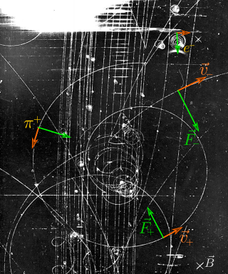
In physics, specifically in electromagnetism, the Lorentz force is the combination of electric and magnetic force on a point charge due to electromagnetic fields. A particle of charge q moving with a velocity v in an electric field E and a magnetic field B experiences a force of

<span class="mw-page-title-main">Potential energy</span> Energy held by an object because of its position relative to other objects

In physics, potential energy is the energy held by an object because of its position relative to other objects, stresses within itself, its electric charge, or other factors. The term potential energy was introduced by the 19th-century Scottish engineer and physicist William Rankine, although it has links to the ancient Greek philosopher Aristotle's concept of potentiality.

<span class="mw-page-title-main">Paramagnetism</span> Weak, attractive magnetism possessed by most elements and some compounds

Paramagnetism is a form of magnetism whereby some materials are weakly attracted by an externally applied magnetic field, and form internal, induced magnetic fields in the direction of the applied magnetic field. In contrast with this behavior, diamagnetic materials are repelled by magnetic fields and form induced magnetic fields in the direction opposite to that of the applied magnetic field. Paramagnetic materials include most chemical elements and some compounds; they have a relative magnetic permeability slightly greater than 1 and hence are attracted to magnetic fields. The magnetic moment induced by the applied field is linear in the field strength and rather weak. It typically requires a sensitive analytical balance to detect the effect and modern measurements on paramagnetic materials are often conducted with a SQUID magnetometer.

<span class="mw-page-title-main">Laplace's equation</span> Second-order partial differential equation

In mathematics and physics, Laplace's equation is a second-order partial differential equation named after Pierre-Simon Laplace, who first studied its properties. This is often written as

<span class="mw-page-title-main">Navier–Stokes equations</span> Equations describing the motion of viscous fluid substances

The Navier–Stokes equations are partial differential equations which describe the motion of viscous fluid substances. They were named after French engineer and physicist Claude-Louis Navier and the Irish physicist and mathematician George Gabriel Stokes. They were developed over several decades of progressively building the theories, from 1822 (Navier) to 1842–1850 (Stokes).

Del, or nabla, is an operator used in mathematics as a vector differential operator, usually represented by the nabla symbol . When applied to a function defined on a one-dimensional domain, it denotes the standard derivative of the function as defined in calculus. When applied to a field, it may denote any one of three operations depending on the way it is applied: the gradient or (locally) steepest slope of a scalar field ; the divergence of a vector field; or the curl (rotation) of a vector field.

In mathematics, the Laplace operator or Laplacian is a differential operator given by the divergence of the gradient of a scalar function on Euclidean space. It is usually denoted by the symbols , (where is the nabla operator), or . In a Cartesian coordinate system, the Laplacian is given by the sum of second partial derivatives of the function with respect to each independent variable. In other coordinate systems, such as cylindrical and spherical coordinates, the Laplacian also has a useful form. Informally, the Laplacian Δf (p) of a function f at a point p measures by how much the average value of f over small spheres or balls centered at p deviates from f (p).

In vector calculus, a conservative vector field is a vector field that is the gradient of some function. A conservative vector field has the property that its line integral is path independent; the choice of path between two points does not change the value of the line integral. Path independence of the line integral is equivalent to the vector field under the line integral being conservative. A conservative vector field is also irrotational; in three dimensions, this means that it has vanishing curl. An irrotational vector field is necessarily conservative provided that the domain is simply connected.

<span class="mw-page-title-main">Scalar potential</span> When potential energy difference depends only on displacement

In mathematical physics, scalar potential, simply stated, describes the situation where the difference in the potential energies of an object in two different positions depends only on the positions, not upon the path taken by the object in traveling from one position to the other. It is a scalar field in three-space: a directionless value (scalar) that depends only on its location. A familiar example is potential energy due to gravity.

<span class="mw-page-title-main">Magnetic moment</span> Magnetic strength and orientation of an object that produces a magnetic field

In electromagnetism, the magnetic moment is the magnetic strength and orientation of a magnet or other object that produces a magnetic field. The magnetic moment is typically expressed as a vector. Examples of objects that have magnetic moments include loops of electric current, permanent magnets, elementary particles, composite particles, various molecules, and many astronomical objects.

In mathematics, Green's identities are a set of three identities in vector calculus relating the bulk with the boundary of a region on which differential operators act. They are named after the mathematician George Green, who discovered Green's theorem.

In electrodynamics, Poynting's theorem is a statement of conservation of energy for electromagnetic fields developed by British physicist John Henry Poynting. It states that in a given volume, the stored energy changes at a rate given by the work done on the charges within the volume, minus the rate at which energy leaves the volume. It is only strictly true in media which is not dispersive, but can be extended for the dispersive case. The theorem is analogous to the work-energy theorem in classical mechanics, and mathematically similar to the continuity equation.

In quantum physics, the spin–orbit interaction is a relativistic interaction of a particle's spin with its motion inside a potential. A key example of this phenomenon is the spin–orbit interaction leading to shifts in an electron's atomic energy levels, due to electromagnetic interaction between the electron's magnetic dipole, its orbital motion, and the electrostatic field of the positively charged nucleus. This phenomenon is detectable as a splitting of spectral lines, which can be thought of as a Zeeman effect product of two relativistic effects: the apparent magnetic field seen from the electron perspective and the magnetic moment of the electron associated with its intrinsic spin. A similar effect, due to the relationship between angular momentum and the strong nuclear force, occurs for protons and neutrons moving inside the nucleus, leading to a shift in their energy levels in the nucleus shell model. In the field of spintronics, spin–orbit effects for electrons in semiconductors and other materials are explored for technological applications. The spin–orbit interaction is at the origin of magnetocrystalline anisotropy and the spin Hall effect.

The following are important identities involving derivatives and integrals in vector calculus.

The derivation of the Navier–Stokes equations as well as its application and formulation for different families of fluids, is an important exercise in fluid dynamics with applications in mechanical engineering, physics, chemistry, heat transfer, and electrical engineering. A proof explaining the properties and bounds of the equations, such as Navier–Stokes existence and smoothness, is one of the important unsolved problems in mathematics.

<span class="mw-page-title-main">Stokes' theorem</span> Theorem in vector calculus

Stokes' theorem, also known as the Kelvin–Stokes theorem after Lord Kelvin and George Stokes, the fundamental theorem for curls or simply the curl theorem, is a theorem in vector calculus on . Given a vector field, the theorem relates the integral of the curl of the vector field over some surface, to the line integral of the vector field around the boundary of the surface. The classical theorem of Stokes can be stated in one sentence: The line integral of a vector field over a loop is equal to the surface integral of its curl over the enclosed surface. It is illustrated in the figure, where the direction of positive circulation of the bounding contour ∂Σ, and the direction n of positive flux through the surface Σ, are related by a right-hand-rule. For the right hand the fingers circulate along ∂Σ and the thumb is directed along n.

Multipole radiation is a theoretical framework for the description of electromagnetic or gravitational radiation from time-dependent distributions of distant sources. These tools are applied to physical phenomena which occur at a variety of length scales - from gravitational waves due to galaxy collisions to gamma radiation resulting from nuclear decay. Multipole radiation is analyzed using similar multipole expansion techniques that describe fields from static sources, however there are important differences in the details of the analysis because multipole radiation fields behave quite differently from static fields. This article is primarily concerned with electromagnetic multipole radiation, although the treatment of gravitational waves is similar.

<span class="mw-page-title-main">Magnetic levitation</span> Suspension of objects by magnetic force.

Magnetic levitation (maglev) or magnetic suspension is a method by which an object is suspended with no support other than magnetic fields. Magnetic force is used to counteract the effects of the gravitational force and any other forces.

References

  1. Weinstock, Robert (1976). "On a fallacious proof of Earnshaw's theorem". American Journal of Physics. 44 (4): 392–393. Bibcode:1976AmJPh..44..392W. doi:10.1119/1.10449.
  2. Gibbs, Philip; Geim, Andre. "Levitation Possible". High Field Magnet Laboratory. Archived from the original on 2012-09-08. Retrieved 2021-05-26.
  3. Earnshaw, S (1842). "On the nature of the molecular forces which regulate the constitution of the luminferous ether". Transactions of the Cambridge Philosophical Society. 7: 97–112.
  4. 1 2 Simon, Martin D.; Heflinger, Lee O.; Ridgway, S.L. (1996). "Spin stabilized magnetic levitation". American Journal of Physics. 65 (4): 286–292. doi:10.1119/1.18488.