
In physics, the Lorentz transformations are a six-parameter family of linear transformations from a coordinate frame in spacetime to another frame that moves at a constant velocity relative to the former. The respective inverse transformation is then parameterized by the negative of this velocity. The transformations are named after the Dutch physicist Hendrik Lorentz.
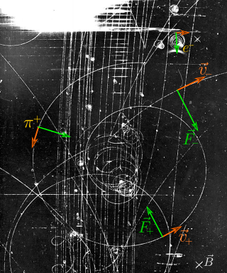
In physics, specifically in electromagnetism, the Lorentz force is the combination of electric and magnetic force on a point charge due to electromagnetic fields. A particle of charge q moving with a velocity v in an electric field E and a magnetic field B experiences a force of
In particle physics, the Dirac equation is a relativistic wave equation derived by British physicist Paul Dirac in 1928. In its free form, or including electromagnetic interactions, it describes all spin-1⁄2 massive particles, called "Dirac particles", such as electrons and quarks for which parity is a symmetry. It is consistent with both the principles of quantum mechanics and the theory of special relativity, and was the first theory to account fully for special relativity in the context of quantum mechanics. It was validated by accounting for the fine structure of the hydrogen spectrum in a completely rigorous way.

The stress–energy tensor, sometimes called the stress–energy–momentum tensor or the energy–momentum tensor, is a tensor physical quantity that describes the density and flux of energy and momentum in spacetime, generalizing the stress tensor of Newtonian physics. It is an attribute of matter, radiation, and non-gravitational force fields. This density and flux of energy and momentum are the sources of the gravitational field in the Einstein field equations of general relativity, just as mass density is the source of such a field in Newtonian gravity.
The Klein–Gordon equation is a relativistic wave equation, related to the Schrödinger equation. It is second-order in space and time and manifestly Lorentz-covariant. It is a differential equation version of the relativistic energy–momentum relation .
In special relativity, a four-vector is an object with four components, which transform in a specific way under Lorentz transformations. Specifically, a four-vector is an element of a four-dimensional vector space considered as a representation space of the standard representation of the Lorentz group, the representation. It differs from a Euclidean vector in how its magnitude is determined. The transformations that preserve this magnitude are the Lorentz transformations, which include spatial rotations and boosts.
Linear elasticity is a mathematical model of how solid objects deform and become internally stressed due to prescribed loading conditions. It is a simplification of the more general nonlinear theory of elasticity and a branch of continuum mechanics.

In classical electromagnetism, magnetic vector potential is the vector quantity defined so that its curl is equal to the magnetic field: . Together with the electric potential φ, the magnetic vector potential can be used to specify the electric field E as well. Therefore, many equations of electromagnetism can be written either in terms of the fields E and B, or equivalently in terms of the potentials φ and A. In more advanced theories such as quantum mechanics, most equations use potentials rather than fields.
In differential geometry, the four-gradient is the four-vector analogue of the gradient from vector calculus.
In electromagnetism, the Lorenz gauge condition or Lorenz gauge is a partial gauge fixing of the electromagnetic vector potential by requiring The name is frequently confused with Hendrik Lorentz, who has given his name to many concepts in this field. The condition is Lorentz invariant. The Lorenz gauge condition does not completely determine the gauge: one can still make a gauge transformation where is the four-gradient and is any harmonic scalar function: that is, a scalar function obeying the equation of a massless scalar field.
In electromagnetism, the electromagnetic tensor or electromagnetic field tensor is a mathematical object that describes the electromagnetic field in spacetime. The field tensor was first used after the four-dimensional tensor formulation of special relativity was introduced by Hermann Minkowski. The tensor allows related physical laws to be written very concisely, and allows for the quantization of the electromagnetic field by Lagrangian formulation described below.

In the physics of gauge theories, gauge fixing denotes a mathematical procedure for coping with redundant degrees of freedom in field variables. By definition, a gauge theory represents each physically distinct configuration of the system as an equivalence class of detailed local field configurations. Any two detailed configurations in the same equivalence class are related by a certain transformation, equivalent to a shear along unphysical axes in configuration space. Most of the quantitative physical predictions of a gauge theory can only be obtained under a coherent prescription for suppressing or ignoring these unphysical degrees of freedom.
In relativistic physics, the electromagnetic stress–energy tensor is the contribution to the stress–energy tensor due to the electromagnetic field. The stress–energy tensor describes the flow of energy and momentum in spacetime. The electromagnetic stress–energy tensor contains the negative of the classical Maxwell stress tensor that governs the electromagnetic interactions.
The covariant formulation of classical electromagnetism refers to ways of writing the laws of classical electromagnetism in a form that is manifestly invariant under Lorentz transformations, in the formalism of special relativity using rectilinear inertial coordinate systems. These expressions both make it simple to prove that the laws of classical electromagnetism take the same form in any inertial coordinate system, and also provide a way to translate the fields and forces from one frame to another. However, this is not as general as Maxwell's equations in curved spacetime or non-rectilinear coordinate systems.
In physics, Maxwell's equations in curved spacetime govern the dynamics of the electromagnetic field in curved spacetime or where one uses an arbitrary coordinate system. These equations can be viewed as a generalization of the vacuum Maxwell's equations which are normally formulated in the local coordinates of flat spacetime. But because general relativity dictates that the presence of electromagnetic fields induce curvature in spacetime, Maxwell's equations in flat spacetime should be viewed as a convenient approximation.
In electromagnetism and applications, an inhomogeneous electromagnetic wave equation, or nonhomogeneous electromagnetic wave equation, is one of a set of wave equations describing the propagation of electromagnetic waves generated by nonzero source charges and currents. The source terms in the wave equations make the partial differential equations inhomogeneous, if the source terms are zero the equations reduce to the homogeneous electromagnetic wave equations. The equations follow from Maxwell's equations.
There are various mathematical descriptions of the electromagnetic field that are used in the study of electromagnetism, one of the four fundamental interactions of nature. In this article, several approaches are discussed, although the equations are in terms of electric and magnetic fields, potentials, and charges with currents, generally speaking.
In quantum mechanics, the Pauli equation or Schrödinger–Pauli equation is the formulation of the Schrödinger equation for spin-½ particles, which takes into account the interaction of the particle's spin with an external electromagnetic field. It is the non-relativistic limit of the Dirac equation and can be used where particles are moving at speeds much less than the speed of light, so that relativistic effects can be neglected. It was formulated by Wolfgang Pauli in 1927. In its linearized form it is known as Lévy-Leblond equation.
The theory of special relativity plays an important role in the modern theory of classical electromagnetism. It gives formulas for how electromagnetic objects, in particular the electric and magnetic fields, are altered under a Lorentz transformation from one inertial frame of reference to another. It sheds light on the relationship between electricity and magnetism, showing that frame of reference determines if an observation follows electric or magnetic laws. It motivates a compact and convenient notation for the laws of electromagnetism, namely the "manifestly covariant" tensor form.
Lagrangian field theory is a formalism in classical field theory. It is the field-theoretic analogue of Lagrangian mechanics. Lagrangian mechanics is used to analyze the motion of a system of discrete particles each with a finite number of degrees of freedom. Lagrangian field theory applies to continua and fields, which have an infinite number of degrees of freedom.


