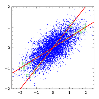
In statistics, the mean squared error (MSE) or mean squared deviation (MSD) of an estimator measures the average of the squares of the errors—that is, the average squared difference between the estimated values and the actual value. MSE is a risk function, corresponding to the expected value of the squared error loss. The fact that MSE is almost always strictly positive is because of randomness or because the estimator does not account for information that could produce a more accurate estimate. In machine learning, specifically empirical risk minimization, MSE may refer to the empirical risk, as an estimate of the true MSE.
In mathematics, a Gaussian function, often simply referred to as a Gaussian, is a function of the base form
In probability theory and statistics, a Gaussian process is a stochastic process, such that every finite collection of those random variables has a multivariate normal distribution. The distribution of a Gaussian process is the joint distribution of all those random variables, and as such, it is a distribution over functions with a continuous domain, e.g. time or space.
In statistics, a generalized linear model (GLM) is a flexible generalization of ordinary linear regression. The GLM generalizes linear regression by allowing the linear model to be related to the response variable via a link function and by allowing the magnitude of the variance of each measurement to be a function of its predicted value.
Random forests or random decision forests is an ensemble learning method for classification, regression and other tasks that operates by constructing a multitude of decision trees at training time. For classification tasks, the output of the random forest is the class selected by most trees. For regression tasks, the mean or average prediction of the individual trees is returned. Random decision forests correct for decision trees' habit of overfitting to their training set.

In statistics, the coefficient of determination, denoted R2 or r2 and pronounced "R squared", is the proportion of the variation in the dependent variable that is predictable from the independent variable(s).
In statistics, ordinary least squares (OLS) is a type of linear least squares method for choosing the unknown parameters in a linear regression model by the principle of least squares: minimizing the sum of the squares of the differences between the observed dependent variable in the input dataset and the output of the (linear) function of the independent variable.
In statistics, the Bayesian information criterion (BIC) or Schwarz information criterion is a criterion for model selection among a finite set of models; models with lower BIC are generally preferred. It is based, in part, on the likelihood function and it is closely related to the Akaike information criterion (AIC).
In statistics, Poisson regression is a generalized linear model form of regression analysis used to model count data and contingency tables. Poisson regression assumes the response variable Y has a Poisson distribution, and assumes the logarithm of its expected value can be modeled by a linear combination of unknown parameters. A Poisson regression model is sometimes known as a log-linear model, especially when used to model contingency tables.
In statistics, the Breusch–Pagan test, developed in 1979 by Trevor Breusch and Adrian Pagan, is used to test for heteroskedasticity in a linear regression model. It was independently suggested with some extension by R. Dennis Cook and Sanford Weisberg in 1983. Derived from the Lagrange multiplier test principle, it tests whether the variance of the errors from a regression is dependent on the values of the independent variables. In that case, heteroskedasticity is present.
Proportional hazards models are a class of survival models in statistics. Survival models relate the time that passes, before some event occurs, to one or more covariates that may be associated with that quantity of time. In a proportional hazards model, the unique effect of a unit increase in a covariate is multiplicative with respect to the hazard rate. For example, taking a drug may halve one's hazard rate for a stroke occurring, or, changing the material from which a manufactured component is constructed may double its hazard rate for failure. Other types of survival models such as accelerated failure time models do not exhibit proportional hazards. The accelerated failure time model describes a situation where the biological or mechanical life history of an event is accelerated.
The cross-entropy (CE) method is a Monte Carlo method for importance sampling and optimization. It is applicable to both combinatorial and continuous problems, with either a static or noisy objective.
Omnibus tests are a kind of statistical test. They test whether the explained variance in a set of data is significantly greater than the unexplained variance, overall. One example is the F-test in the analysis of variance. There can be legitimate significant effects within a model even if the omnibus test is not significant. For instance, in a model with two independent variables, if only one variable exerts a significant effect on the dependent variable and the other does not, then the omnibus test may be non-significant. This fact does not affect the conclusions that may be drawn from the one significant variable. In order to test effects within an omnibus test, researchers often use contrasts.
The root mean square deviation (RMSD) or root mean square error (RMSE) is either one of two closely related and frequently used measures of the differences between true or predicted values on the one hand and observed values or an estimator on the other.
In probability and statistics, the Tweedie distributions are a family of probability distributions which include the purely continuous normal, gamma and inverse Gaussian distributions, the purely discrete scaled Poisson distribution, and the class of compound Poisson–gamma distributions which have positive mass at zero, but are otherwise continuous. Tweedie distributions are a special case of exponential dispersion models and are often used as distributions for generalized linear models.
In statistics, identifiability is a property which a model must satisfy for precise inference to be possible. A model is identifiable if it is theoretically possible to learn the true values of this model's underlying parameters after obtaining an infinite number of observations from it. Mathematically, this is equivalent to saying that different values of the parameters must generate different probability distributions of the observable variables. Usually the model is identifiable only under certain technical restrictions, in which case the set of these requirements is called the identification conditions.

In statistics, errors-in-variables models or measurement error models are regression models that account for measurement errors in the independent variables. In contrast, standard regression models assume that those regressors have been measured exactly, or observed without error; as such, those models account only for errors in the dependent variables, or responses.
Taylor's power law is an empirical law in ecology that relates the variance of the number of individuals of a species per unit area of habitat to the corresponding mean by a power law relationship. It is named after the ecologist who first proposed it in 1961, Lionel Roy Taylor (1924–2007). Taylor's original name for this relationship was the law of the mean. The name Taylor's law was coined by Southwood in 1966.
In statistics, the variance function is a smooth function that depicts the variance of a random quantity as a function of its mean. The variance function is a measure of heteroscedasticity and plays a large role in many settings of statistical modelling. It is a main ingredient in the generalized linear model framework and a tool used in non-parametric regression, semiparametric regression and functional data analysis. In parametric modeling, variance functions take on a parametric form and explicitly describe the relationship between the variance and the mean of a random quantity. In a non-parametric setting, the variance function is assumed to be a smooth function.
Alternating conditional expectations (ACE) is an algorithm to find the optimal transformations between the response variable and predictor variables in regression analysis.


