Definition
The flow velocity u of a fluid is a vector field

which gives the velocity of an element of fluid at a position and time


The flow speed q is the length of the flow velocity vector [3]

and is a scalar field.
In continuum mechanics the flow velocity in fluid dynamics, also macroscopic velocity [1] [2] in statistical mechanics, or drift velocity in electromagnetism, is a vector field used to mathematically describe the motion of a continuum. The length of the flow velocity vector is scalar, the flow speed. It is also called velocity field; when evaluated along a line, it is called a velocity profile (as in, e.g., law of the wall).
The flow velocity u of a fluid is a vector field
which gives the velocity of an element of fluid at a position and time
The flow speed q is the length of the flow velocity vector [3]
and is a scalar field.
The flow velocity of a fluid effectively describes everything about the motion of a fluid. Many physical properties of a fluid can be expressed mathematically in terms of the flow velocity. Some common examples follow:
The flow of a fluid is said to be steady if does not vary with time. That is if
If a fluid is incompressible the divergence of is zero:
That is, if is a solenoidal vector field.
A flow is irrotational if the curl of is zero:
That is, if is an irrotational vector field.
A flow in a simply-connected domain which is irrotational can be described as a potential flow, through the use of a velocity potential with If the flow is both irrotational and incompressible, the Laplacian of the velocity potential must be zero:
The vorticity, , of a flow can be defined in terms of its flow velocity by
If the vorticity is zero, the flow is irrotational.
If an irrotational flow occupies a simply-connected fluid region then there exists a scalar field such that
The scalar field is called the velocity potential for the flow. (See Irrotational vector field.)
In many engineering applications the local flow velocity vector field is not known in every point and the only accessible velocity is the bulk velocity or average flow velocity (with the usual dimension of length per time), defined as the quotient between the volume flow rate (with dimension of cubed length per time) and the cross sectional area (with dimension of square length):

The Navier–Stokes equations are partial differential equations which describe the motion of viscous fluid substances. They were named after French engineer and physicist Claude-Louis Navier and the Irish physicist and mathematician George Gabriel Stokes. They were developed over several decades of progressively building the theories, from 1822 (Navier) to 1842–1850 (Stokes).
In fluid dynamics, potential flow is the ideal flow pattern of an inviscid fluid. Potential flows are described and determined by mathematical methods.
In continuum mechanics, vorticity is a pseudovector field that describes the local spinning motion of a continuum near some point, as would be seen by an observer located at that point and traveling along with the flow. It is an important quantity in the dynamical theory of fluids and provides a convenient framework for understanding a variety of complex flow phenomena, such as the formation and motion of vortex rings.
The vorticity equation of fluid dynamics describes the evolution of the vorticity ω of a particle of a fluid as it moves with its flow; that is, the local rotation of the fluid. The governing equation is:
The stream function is defined for incompressible (divergence-free) flows in two dimensions – as well as in three dimensions with axisymmetry. The flow velocity components can be expressed as the derivatives of the scalar stream function. The stream function can be used to plot streamlines, which represent the trajectories of particles in a steady flow. The two-dimensional Lagrange stream function was introduced by Joseph Louis Lagrange in 1781. The Stokes stream function is for axisymmetrical three-dimensional flow, and is named after George Gabriel Stokes.
In vector calculus, a conservative vector field is a vector field that is the gradient of some function. A conservative vector field has the property that its line integral is path independent; the choice of path between two points does not change the value of the line integral. Path independence of the line integral is equivalent to the vector field under the line integral being conservative. A conservative vector field is also irrotational; in three dimensions, this means that it has vanishing curl. An irrotational vector field is necessarily conservative provided that the domain is simply connected.

In mathematical physics, scalar potential, simply stated, describes the situation where the difference in the potential energies of an object in two different positions depends only on the positions, not upon the path taken by the object in traveling from one position to the other. It is a scalar field in three-space: a directionless value (scalar) that depends only on its location. A familiar example is potential energy due to gravity.
In physics, chemistry and biology, a potential gradient is the local rate of change of the potential with respect to displacement, i.e. spatial derivative, or gradient. This quantity frequently occurs in equations of physical processes because it leads to some form of flux.
In fluid mechanics, the Taylor–Proudman theorem states that when a solid body is moved slowly within a fluid that is steadily rotated with a high angular velocity , the fluid velocity will be uniform along any line parallel to the axis of rotation. must be large compared to the movement of the solid body in order to make the Coriolis force large compared to the acceleration terms.

Stokes flow, also named creeping flow or creeping motion, is a type of fluid flow where advective inertial forces are small compared with viscous forces. The Reynolds number is low, i.e. . This is a typical situation in flows where the fluid velocities are very slow, the viscosities are very large, or the length-scales of the flow are very small. Creeping flow was first studied to understand lubrication. In nature, this type of flow occurs in the swimming of microorganisms and sperm. In technology, it occurs in paint, MEMS devices, and in the flow of viscous polymers generally.
A velocity potential is a scalar potential used in potential flow theory. It was introduced by Joseph-Louis Lagrange in 1788.
In fluid mechanics, potential vorticity (PV) is a quantity which is proportional to the dot product of vorticity and stratification. This quantity, following a parcel of air or water, can only be changed by diabatic or frictional processes. It is a useful concept for understanding the generation of vorticity in cyclogenesis, especially along the polar front, and in analyzing flow in the ocean.

The Navier–Stokes existence and smoothness problem concerns the mathematical properties of solutions to the Navier–Stokes equations, a system of partial differential equations that describe the motion of a fluid in space. Solutions to the Navier–Stokes equations are used in many practical applications. However, theoretical understanding of the solutions to these equations is incomplete. In particular, solutions of the Navier–Stokes equations often include turbulence, which remains one of the greatest unsolved problems in physics, despite its immense importance in science and engineering.
The derivation of the Navier–Stokes equations as well as its application and formulation for different families of fluids, is an important exercise in fluid dynamics with applications in mechanical engineering, physics, chemistry, heat transfer, and electrical engineering. A proof explaining the properties and bounds of the equations, such as Navier–Stokes existence and smoothness, is one of the important unsolved problems in mathematics.
In fluid dynamics, The projection method is an effective means of numerically solving time-dependent incompressible fluid-flow problems. It was originally introduced by Alexandre Chorin in 1967 as an efficient means of solving the incompressible Navier-Stokes equations. The key advantage of the projection method is that the computations of the velocity and the pressure fields are decoupled.

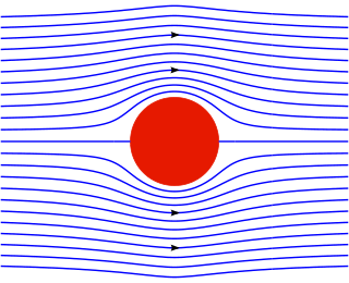
In mathematics, potential flow around a circular cylinder is a classical solution for the flow of an inviscid, incompressible fluid around a cylinder that is transverse to the flow. Far from the cylinder, the flow is unidirectional and uniform. The flow has no vorticity and thus the velocity field is irrotational and can be modeled as a potential flow. Unlike a real fluid, this solution indicates a net zero drag on the body, a result known as d'Alembert's paradox.
Irrotational flow occurs where the curl of the velocity of the fluid is zero everywhere. That is when
In fluid mechanics, Kelvin's minimum energy theorem states that the steady irrotational motion of an incompressible fluid occupying a simply connected region has less kinetic energy than any other motion with the same normal component of velocity at the boundary .
In fluid dynamics, Lamb vector is the cross product of vorticity vector and velocity vector of the flow field, named after the physicist Horace Lamb. The Lamb vector is defined as
In the larger context of the Navier-Stokes equations, elementary flows are a collection of basic flows from which it is possible to construct more complex flows with different techniques. In this article the term flows is used interchangeably to the term solutions due to historical reasons.
{{cite book}}: CS1 maint: location missing publisher (link){{cite book}}: CS1 maint: location missing publisher (link)| Authority control databases: National |
|---|


