Genetic distance

Last updated
Figure 1: Genetic distance map by Cavalli-Sforza et al. (1994) The history and geography of human genes Luigi Luca Cavalli-Sforza map genetic.png
Figure 1: Genetic distance map by Cavalli-Sforza et al. (1994)

Genetic distance is a measure of the genetic divergence between species or between populations within a species, whether the distance measures time from common ancestor or degree of differentiation. [2] Populations with many similar alleles have small genetic distances. This indicates that they are closely related and have a recent common ancestor.

Contents

Genetic distance is useful for reconstructing the history of populations, such as the multiple human expansions out of Africa. [3] It is also used for understanding the origin of biodiversity. For example, the genetic distances between different breeds of domesticated animals are often investigated in order to determine which breeds should be protected to maintain genetic diversity. [4]

Biological foundation

Life on earth began from very simple unicellular organisms evolving into most complex multicellular organisms through the course of over three billion years. [5] Creating a comprehensive tree of life that represents all the organisms that have ever lived on earth is important for understanding the evolution of life in the face of all challenges faced by living organisms to deal with similar challenges in future. Evolutionary biologists have attempted to create evolutionary or phylogenetic trees encompassing as many organisms as possible based on the available resources. Fossil dating and molecular clock are the two means of generating evolutionary history of living organisms. Fossil record is random, incomplete and does not provide a continuous chain of events like a movie with missing frames cannot tell the whole plot of the movie. [5]

Molecular clocks on the other hand are specific sequences of DNA, RNA or proteins (amino acids) that are used to determine at molecular level the similarities and differences among species, to find out the timeline of divergence, [6] and to trace back the common ancestor of species based on the mutation rates and sequence changes being accumulated in those specific sequences. [6] The primary driver of evolution is the mutation or changes in genes and accounting for those changes overtime determines the approximate genetic distance between species. These specific molecular clocks are fairly conserved across a range of species and have a constant rate of mutation like a clock and are calibrated based on evolutionary events (fossil records). For example, gene for alpha-globin (constituent of hemoglobin) mutates at a rate of 0.56 per base pair per billion years. [6] The molecular clock can fill those gaps created by missing fossil records.

In the genome of an organism, each gene is located at a specific place called the locus for that gene. Allelic variations at these loci cause phenotypic variation within species (e.g. hair colour, eye colour). However, most alleles do not have an observable impact on the phenotype. Within a population new alleles generated by mutation either die out or spread throughout the population. When a population is split into different isolated populations (by either geographical or ecological factors), mutations that occur after the split will be present only in the isolated population. Random fluctuation of allele frequencies also produces genetic differentiation between populations. This process is known as genetic drift. By examining the differences between allele frequencies between the populations and computing genetic distance, we can estimate how long ago the two populations were separated. [7]

Let’s suppose a sequence of DNA or a hypothetical gene that has mutation rate of one base per 10 million years. Using this sequence of DNA, the divergence of two different species or genetic distance between two different species can be determined by counting the number of base pair differences among them. For example, in Figure 2 a difference of 4 bases in the hypothetical sequence among those two species would indicate that they diverged 40 million years ago, and their common ancestor would have lived at least 20 million years ago before their divergence. Based on molecular clock, the equation below can be used to calculate the time since divergence. [8]

Number of mutation ÷ Mutation per year (rate of mutation) = time since divergence

Figure 2: Divergence timeline between two hypothetical species. Divergence timeline between species.png
Figure 2: Divergence timeline between two hypothetical species.

Process of determining genetic distance

Recent advancement in sequencing technology and the availability of comprehensive genomic databases and bioinformatics tools that are capable of storing and processing colossal amount of data generated by the advanced sequencing technology has tremendously improved evolutionary studies and the understanding of evolutionary relationships among species. [9] [10]

Markers for genetic distance

Different biomolecular markers such DNA, RNA and amino acid sequences (protein) can be used for determining the genetic distance. [11] [12]

The selection criteria [13] of appropriate biomarker for genetic distance entails the following three steps:

  1. choice of variability
  2. choice of specific region of DNA or RNA
  3. the use of technique

The choice of variability depends on the intended outcome. For example, very high level of variability is recommended for demographic studies and parentage analyses, medium to high variability for comparing distinct populations, and moderate to very low variability is recommended for phylogenetic studies. [13] The genomic localization and ploidy of the marker is also an important factor. For example, the gene copy numbe r is inversely proportional to the robustness with haploid genome (mitochondrial DNA) more prone to genetic drift than diploid genome (nuclear DNA).

The choice and examples of molecular markers for evolutionary biology studies. [13]

Biological issues/biodiversity levelLevel of variabilityNature of information requiredExamples of most used markers
Intra-populationPopulation structure, reproduction systemMedium to high(N) codominant

loci = (Multilocus)

genotype

Microsatellites, allozymes
Fingerprinting. parentage analysis Very highCodominant loci or numerous dominant lociMicrosatellites (RAPD, AFLP)
DemographyMedium to highAllele frequency in samples taken at different timesAllozymes, Microsatellites
Demographic history Medium to highAllele frequency + evolutionary relationships Mt-DNA sequences
Inter-population Phylogeography, definition of evolutionary significant units (population structure)Medium to highAllele frequency in each populationAllozymes, microsatellites (risk of size homoplasy)
Bio-conservation MediumAllele evolutionary relationshipsMt-DNA (if variable enough)
Inter-specificClose species ca. 1%/my No variability within species if possibleSequences of Mt-DNA, ITS rDNA

Application of genetic distance

Evolutionary forces affecting genetic distance

Evolutionary forces such as mutation, genetic drift, natural selection, and gene flow drive the process of evolution and genetic diversity. All these forces play significant role in genetic distance within and among species. [19]

Measures

Peripatric Speciation.svg
Figure 3: Image depicts speciation stemmed from geographic isolation where a starting population is separated. Over vast amounts of time, isolated groups of a particular taxa may diverge into distinct species.

Different statistical measures exist that aim to quantify genetic deviation between populations or species. By utilizing assumptions gained from experimental analysis of evolutionary forces, a model that more accurately suits a given experiment can be selected to study a genetic group. Additionally, comparing how well different metrics model certain population features such as isolation can identify metrics that are more suited for understanding newly studied groups [20] The most commonly used genetic distance metrics are Nei's genetic distance, [7] Cavalli-Sforza and Edwards measure, [21] and Reynolds, Weir and Cockerham's genetic distance. [22]

Jukes-Cantor Distance

One of the most basic and straight forward distance measures is Jukes-Cantor distance. This measure is constructed based on the assumption that no insertions or deletions occurred, all substitutions are independent, and that each nucleotide change is equally likely. With these presumptions, we can obtain the following equation: [23]

where is the Jukes-Cantor distance between two sequences A, and B, and being the dissimilarity between the two sequences.

Nei's standard genetic distance

In 1972, Masatoshi Nei published what came to be known as Nei's standard genetic distance. This distance has the nice property that if the rate of genetic change (amino acid substitution) is constant per year or generation then Nei's standard genetic distance (D) increases in proportion to divergence time. This measure assumes that genetic differences are caused by mutation and genetic drift. [7]

This distance can also be expressed in terms of the arithmetic mean of gene identity. Let be the probability for the two members of population having the same allele at a particular locus and be the corresponding probability in population . Also, let be the probability for a member of and a member of having the same allele. Now let , and represent the arithmetic mean of , and over all loci, respectively. In other words,

where is the total number of loci examined. [24]

Nei's standard distance can then be written as [7]

Cavalli-Sforza chord distance

In 1967 Luigi Luca Cavalli-Sforza and A. W. F. Edwards published this measure. It assumes that genetic differences arise due to genetic drift only. One major advantage of this measure is that the populations are represented in a hypersphere, the scale of which is one unit per gene substitution. The chord distance in the hyperdimensional sphere is given by [2] [21]

Some authors drop the factor to simplify the formula at the cost of losing the property that the scale is one unit per gene substitution.

Reynolds, Weir, and Cockerham's genetic distance

In 1983, this measure was published by John Reynolds, Bruce Weir and C. Clark Cockerham. This measure assumes that genetic differentiation occurs only by genetic drift without mutations. It estimates the coancestry coefficient which provides a measure of the genetic divergence by: [22]

Kimura 2 Parameter distance

Figure 4: A diagram showing the relationship between DNA base-pairs and the type of mutation needed to convert each base to another based on the Kimura 2 parameter substitution model. Kimura two parameter substitution model.png
Figure 4: A diagram showing the relationship between DNA base-pairs and the type of mutation needed to convert each base to another based on the Kimura 2 parameter substitution model.

The Kimura two parameter model (K2P) was developed in 1980 by Japanese biologist Motoo Kimura. It is compatible with the neutral theory of evolution, which was also developed by the same author. As depicted in Figure 4, this measure of genetic distance accounts for the type of mutation occurring, namely whether it is a transition (i.e. purine to purine or pyrimidine to pyrimidine) or a transversion (i.e. purine to pyrimidine or vice versa). With this information, the following formula can be derived:

where P is and Q is , with being the number of transition type conversions, being the number of transversion type conversions, and being the number of nucleotides sites compared. [25]

It is worth noting when transition and transversion type substitutions have an equal chance of occurring, and is assumed to equal , then the above formula can be reduced down to the Jukes Cantor model. In practice however, is typically larger than . [25]

It has been shown that while K2P works well in classifying distantly-related species, it is not always the best choice for comparing closely-related species. In these cases, it may be better to use p-distance instead. [26]

Kimura 3 Parameter distance

Figure 5: A diagram showing the relationship between DNA base-pairs and the type of mutation needed to convert each base to another based on the Kimura 3 parameter substitution model. Kimura three parameter substitution model.png
Figure 5: A diagram showing the relationship between DNA base-pairs and the type of mutation needed to convert each base to another based on the Kimura 3 parameter substitution model.

The Kimura three parameter (K3P) model was first published in 1981. This measure assumes three rates of substitution when nucleotides mutate, which can be seen in Figure 5. There is one rate for transition type mutations, one rate for transversion type mutations to corresponding bases (e.g. G to C; transversion type 1 in the figure), and one rate for transversion type mutations to non-corresponding bases (e.g. G to T; transversion type 2 in the figure).

With these rates of substitution, the following formula can be derived:

where is the probability of a transition type mutation, is the probability of a transversion type mutation to a corresponding base, and is the probability of a transversion type mutation to a non-corresponding base. When and are assumed to be equal, this reduces down to the Kimura 2 parameter distance. [27]

Other measures

Many other measures of genetic distance have been proposed with varying success.

Nei's DA distance 1983

Nei's DA distance was created by Masatoshi Nei, a Japanese-American biologist in 1983. This distance assumes that genetic differences arise due to mutation and genetic drift, but this distance measure is known to give more reliable population trees than other distances particularly for microsatellite DNA data. This method is not ideal in cases where natural selection plays a significant role in a populations genetics. [28] [29]

: Nei's DA distance, the genetic distance between populations X and Y

: A locus or gene studied with being the sum of loci or genes

and : The frequencies of allele u in populations X and Y, respectively

L: The total number of loci examined

Euclidean distance

Figure 6: Euclidean genetic distance between 51 worldwide human populations, calculated using 289,160 SNPs. Dark red is the most similar pair and dark blue is the most distant pair. Genetic similarities between 51 worldwide human populations (Euclidean genetic distance using 289,160 SNPs).png
Figure 6: Euclidean genetic distance between 51 worldwide human populations, calculated using 289,160 SNPs. Dark red is the most similar pair and dark blue is the most distant pair.

Euclidean distance is a formula brought about from Euclid's Elements, a 13 book set detailing the foundation of all euclidean mathematics. The foundational principles outlined in these works is used not only in euclidean spaces but expanded upon by Issac Newton and Gottfried Leibniz in isolated pursuits to create calculus. [31] The euclidean distance formula is used to convey, as simply as possible, the genetic dissimilarity between populations, with a larger distance indicating greater dissimilarity. [32] As seen in figure 6, this method can be visualized in a graphical manner, this is due to the work of René Descartes who created the fundamental principle of analytic geometry, or the cartesian coordinate system. In an interesting example of historical repetitions, René Descartes was not the only one who discovered the fundamental principle of analytical geometry, this principle was as discovered in an isolated pursuit by Pierre de Fermat who left his work unpublished. [33] [34]

[2]

: Euclidean genetic distance between populations X and Y

and : Allele frequencies at locus u in populations X and Y, respectively

Goldstein distance 1995

It was specifically developed for microsatellite markers and is based on the stepwise-mutation model (SMM). The Goldstein distance formula is modeled in such a way that expected value will increase linearly with time, this property is maintained even when the assumptions of single-step mutations and symmetrical mutation rate are violated. Goldstein distance is derived from the average square distance model, of which Goldstein was also a contributor. [35]

: Goldstein genetic distance between populations X and Y
and : Mean allele sizes in populations X and Y
L: Total number of microsatallite loci examined

Nei's minimum genetic distance 1973

This calculation represents the minimum amount of codon differences for each locus. [36] The measurement is based on the assumption that genetic differences arise due to mutation and genetic drift. [37]

: Minimum amount of codon difference per locus

and : Average probability of two members of the X population having the same allele

: Average probability of members of the X and Y populations having the same allele

Czekanowski (Manhattan) Distance

Figure 7: Representation of path between points that is calculated for the Czekanwski (Manhattan) distance formula. Example of Multi-Agent Path Finding in a grid environment.png
Figure 7: Representation of path between points that is calculated for the Czekanwski (Manhattan) distance formula.

Similar to Euclidean distance, Czekanowski distance involves calculated the distance between points of allele frequency that are graphed on an axis created by . However, Czekanowski assumes a direct path is not available and sums the sides of the triangle formed by the data points instead of finding the hypotenuse. This formula is nicknamed the Manhattan distance because its methodology is similar to the nature of the New York City burrow. Manhattan is mainly built on a grid system requiring resentence to only make 90 degree turns during travel, which parallels the thinking of the formula.

and : Allele frequencies at locus u in populations X and Y, respectively

and : X-axis value of the frequency of an allele for X and Y populations

and : Y-axis value of the frequency of an allele for X and Y populations

Roger's Distance 1972

Figure 8: Representation of path between points that is calculated for the Roger's distance formula. Cube-Diagonals.svg
Figure 8: Representation of path between points that is calculated for the Roger's distance formula.

Similar to Czekanowski distance, Roger's distance involves calculating the distance between points of allele frequency. However, this method takes the direct distance between the points.

[38]

and : Allele frequencies at locus u in populations X and Y, respectively

: Total number of microsatallite loci examined

Limitations of Simple Distance Formulas

While these formulas are easy and quick calculations to make, the information that is provided gives limited information. The results of these formulas do not account for the potential effects of the number of codon changes between populations, or separation time between populations. [39]

Fixation Index

A commonly used measure of genetic distance is the fixation index (FST) which varies between 0 and 1. A value of 0 indicates that two populations are genetically identical (minimal or no genetic diversity between the two populations) whereas a value of 1 indicates that two populations are genetically different (maximum genetic diversity between the two populations). No mutation is assumed. Large populations between which there is much migration, for example, tend to be little differentiated whereas small populations between which there is little migration tend to be greatly differentiated. FST is a convenient measure of this differentiation, and as a result FST and related statistics are among the most widely used descriptive statistics in population and evolutionary genetics. But FST is more than a descriptive statistic and measure of genetic differentiation. FST is directly related to the Variance in allele frequency among populations and conversely to the degree of resemblance among individuals within populations. If FST is small, it means that allele frequencies within each population are very similar; if it is large, it means that allele frequencies are very different.

Software

See also

Related Research Articles

An allele, or allelomorph, is a variant of the sequence of nucleotides at a particular location, or locus, on a DNA molecule.

Genetic drift, also known as random genetic drift, allelic drift or the Wright effect, is the change in the frequency of an existing gene variant (allele) in a population due to random chance.

<span class="mw-page-title-main">Neutral theory of molecular evolution</span> Theory of evolution by changes at the molecular level

The neutral theory of molecular evolution holds that most evolutionary changes occur at the molecular level, and most of the variation within and between species are due to random genetic drift of mutant alleles that are selectively neutral. The theory applies only for evolution at the molecular level, and is compatible with phenotypic evolution being shaped by natural selection as postulated by Charles Darwin.

Fitness is a quantitative representation of individual reproductive success. It is also equal to the average contribution to the gene pool of the next generation, made by the same individuals of the specified genotype or phenotype. Fitness can be defined either with respect to a genotype or to a phenotype in a given environment or time. The fitness of a genotype is manifested through its phenotype, which is also affected by the developmental environment. The fitness of a given phenotype can also be different in different selective environments.

Population genetics is a subfield of genetics that deals with genetic differences within and among populations, and is a part of evolutionary biology. Studies in this branch of biology examine such phenomena as adaptation, speciation, and population structure.

Allele frequency, or gene frequency, is the relative frequency of an allele at a particular locus in a population, expressed as a fraction or percentage. Specifically, it is the fraction of all chromosomes in the population that carry that allele over the total population or sample size. Microevolution is the change in allele frequencies that occurs over time within a population.

Genetic linkage is the tendency of DNA sequences that are close together on a chromosome to be inherited together during the meiosis phase of sexual reproduction. Two genetic markers that are physically near to each other are unlikely to be separated onto different chromatids during chromosomal crossover, and are therefore said to be more linked than markers that are far apart. In other words, the nearer two genes are on a chromosome, the lower the chance of recombination between them, and the more likely they are to be inherited together. Markers on different chromosomes are perfectly unlinked, although the penetrance of potentially deleterious alleles may be influenced by the presence of other alleles, and these other alleles may be located on other chromosomes than that on which a particular potentially deleterious allele is located.

<span class="mw-page-title-main">Genetic diversity</span> Total number of genetic characteristics in a species

Genetic diversity is the total number of genetic characteristics in the genetic makeup of a species, it ranges widely from the number of species to differences within species and can be attributed to the span of survival for a species. It is distinguished from genetic variability, which describes the tendency of genetic characteristics to vary.

<span class="mw-page-title-main">Linkage disequilibrium</span> Allele association in population genetics

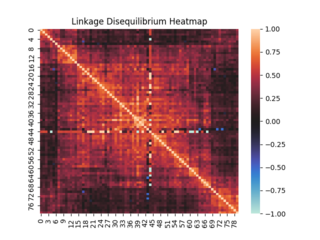
In population genetics, linkage disequilibrium (LD) is a measure of non-random association between segments of DNA (alleles) at different positions on the chromosome (loci) in a given population based on a comparison between the frequency at which two alleles are detected together at the same loci and the frequencies at which each allele is detected at that loci overall, whether it occurs with or without the other allele of interest. Loci are said to be in linkage disequilibrium when the frequency of being detected together is higher or lower than expected if the loci were independent and associated randomly.

Nucleotide diversity is a concept in molecular genetics which is used to measure the degree of polymorphism within a population.

The effective population size (Ne) is size of an idealised population would experience the same rate of genetic drift or increase in inbreeding as in the real population. Idealised populations are based on unrealistic but convenient assumptions including random mating, simultaneous birth of each new generation, constant population size. For most quantities of interest and most real populations, Ne is smaller than the census population size N of a real population. The same population may have multiple effective population sizes for different properties of interest, including genetic drift and inbreeding.

<span class="mw-page-title-main">Conservation genetics</span> Interdisciplinary study of extinction avoidance

Conservation genetics is an interdisciplinary subfield of population genetics that aims to understand the dynamics of genes in a population for the purpose of natural resource management, conservation of genetic diversity, and the prevention of species extinction. Scientists involved in conservation genetics come from a variety of fields including population genetics, research in natural resource management, molecular ecology, molecular biology, evolutionary biology, and systematics. The genetic diversity within species is one of the three fundamental components of biodiversity, so it is an important consideration in the wider field of conservation biology.

Genetic load is the difference between the fitness of an average genotype in a population and the fitness of some reference genotype, which may be either the best present in a population, or may be the theoretically optimal genotype. The average individual taken from a population with a low genetic load will generally, when grown in the same conditions, have more surviving offspring than the average individual from a population with a high genetic load. Genetic load can also be seen as reduced fitness at the population level compared to what the population would have if all individuals had the reference high-fitness genotype. High genetic load may put a population in danger of extinction.

Genetic hitchhiking, also called genetic draft or the hitchhiking effect, is when an allele changes frequency not because it itself is under natural selection, but because it is near another gene that is undergoing a selective sweep and that is on the same DNA chain. When one gene goes through a selective sweep, any other nearby polymorphisms that are in linkage disequilibrium will tend to change their allele frequencies too. Selective sweeps happen when newly appeared mutations are advantageous and increase in frequency. Neutral or even slightly deleterious alleles that happen to be close by on the chromosome 'hitchhike' along with the sweep. In contrast, effects on a neutral locus due to linkage disequilibrium with newly appeared deleterious mutations are called background selection. Both genetic hitchhiking and background selection are stochastic (random) evolutionary forces, like genetic drift.

<span class="mw-page-title-main">Fixation index</span> Measure of population differentiation

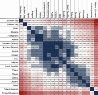
The fixation index (FST) is a measure of population differentiation due to genetic structure. It is frequently estimated from genetic polymorphism data, such as single-nucleotide polymorphisms (SNP) or microsatellites. Developed as a special case of Wright's F-statistics, it is one of the most commonly used statistics in population genetics. Its values range from 0 to 1, with 0.15 being substantially differentiated and 1 being complete differentiation.

<span class="mw-page-title-main">Masatoshi Nei</span> Japanese-American geneticist (1931–2023)

Masatoshi Nei was a Japanese-born American evolutionary biologist.

In population genetics, fixation is the change in a gene pool from a situation where there exists at least two variants of a particular gene (allele) in a given population to a situation where only one of the alleles remains. That is, the allele becomes fixed. In the absence of mutation or heterozygote advantage, any allele must eventually either be lost completely from the population, or fixed, i.e. permanently established at 100% frequency in the population. Whether a gene will ultimately be lost or fixed is dependent on selection coefficients and chance fluctuations in allelic proportions. Fixation can refer to a gene in general or particular nucleotide position in the DNA chain (locus).

Population structure is the presence of a systematic difference in allele frequencies between subpopulations. In a randomly mating population, allele frequencies are expected to be roughly similar between groups. However, mating tends to be non-random to some degree, causing structure to arise. For example, a barrier like a river can separate two groups of the same species and make it difficult for potential mates to cross; if a mutation occurs, over many generations it can spread and become common in one subpopulation while being completely absent in the other.

The Infinite sites model (ISM) is a mathematical model of molecular evolution first proposed by Motoo Kimura in 1969. Like other mutation models, the ISM provides a basis for understanding how mutation develops new alleles in DNA sequences. Using allele frequencies, it allows for the calculation of heterozygosity, or genetic diversity, in a finite population and for the estimation of genetic distances between populations of interest.

This glossary of genetics and evolutionary biology is a list of definitions of terms and concepts used in the study of genetics and evolutionary biology, as well as sub-disciplines and related fields, with an emphasis on classical genetics, quantitative genetics, population biology, phylogenetics, speciation, and systematics. Overlapping and related terms can be found in Glossary of cellular and molecular biology, Glossary of ecology, and Glossary of biology.

References

  1. Cavalli-Sforza, L.L., Menozzi, P. & Piazza, A. (1994). The History and Geography of Human Genes. New Jersey: Princeton University Press.
  2. 1 2 3 Nei, M. (1987). "Chapter 9". Molecular Evolutionary Genetics. New York: Columbia University Press.
  3. Ramachandran S, Deshpande O, Roseman CC, Rosenberg NA, Feldman MW, Cavalli-Sforza LL (November 2005). "Support from the relationship of genetic and geographic distance in human populations for a serial founder effect originating in Africa". Proc Natl Acad Sci U S A. 102 (44): 15942–7. Bibcode:2005PNAS..10215942R. doi: 10.1073/pnas.0507611102 . PMC   1276087 . PMID   16243969.
  4. Ruane J (1999). "A critical review of the value of genetic distance studies in conservation of animal genetic resources". Journal of Animal Breeding and Genetics. 116 (5): 317–323. doi:10.1046/j.1439-0388.1999.00205.x.
  5. 1 2 #author.fullName}. "Timeline: The evolution of life". New Scientist. Retrieved 2024-04-17.{{cite web}}: |last= has generic name (help)
  6. 1 2 3 "Molecular clocks". evolution.berkeley.edu. Retrieved 2024-04-18.
  7. 1 2 3 4 Nei, M. (1972). "Genetic distance between populations". Am. Nat. 106 (949): 283–292. doi:10.1086/282771. S2CID   55212907.
  8. Cheng, Eric C.K. (2024-01-18), "Crafting future pedagogies through Lesson Study", Implementing a 21st Century Competency-Based Curriculum Through Lesson Study, London: Routledge, pp. 3–18, ISBN   978-1-003-37410-7 , retrieved 2024-04-18
  9. Koboldt, Daniel C.; Steinberg, Karyn Meltz; Larson, David E.; Wilson, Richard K.; Mardis, Elaine R. (2013-09-26). "The Next-Generation Sequencing Revolution and Its Impact on Genomics". Cell. 155 (1): 27–38. doi:10.1016/j.cell.2013.09.006. PMC   3969849 .
  10. Hudson, Matthew E. (January 2008). "Sequencing breakthroughs for genomic ecology and evolutionary biology". Molecular Ecology Resources. 8 (1): 3–17. doi:10.1111/j.1471-8286.2007.02019.x. ISSN   1755-098X.
  11. Kartavtsev, Yuri Phedorovich (2021-05-20). "Some Examples of the Use of Molecular Markers for Needs of Basic Biology and Modern Society". Animals. 11 (5): 1473. doi: 10.3390/ani11051473 . ISSN   2076-2615. PMC   8160991 .
  12. Bhandari, Vaibhav; Naushad, Hafiz S.; Gupta, Radhey S. (2012). "Protein based molecular markers provide reliable means to understand prokaryotic phylogeny and support Darwinian mode of evolution". Frontiers in Cellular and Infection Microbiology. 2. doi: 10.3389/fcimb.2012.00098 . ISSN   2235-2988. PMC   3417386 .
  13. 1 2 3 Anne, Chenuil (May 2006). "Choosing the right molecular genetic markers for studying biodiversity: from molecular evolution to practical aspects". Genetica. 127 (1–3): 101–120. doi:10.1007/s10709-005-2485-1. ISSN   0016-6707.
  14. Scutari, Marco; Mackay, Ian; Balding, David (2016-09-02). Hickey, John Micheal (ed.). "Using Genetic Distance to Infer the Accuracy of Genomic Prediction". PLOS Genetics. 12 (9): e1006288. arXiv: 1509.00415 . doi: 10.1371/journal.pgen.1006288 . ISSN   1553-7404.
  15. Shin, Caren P.; Allmon, Warren D. (September 2023). "How we study cryptic species and their biological implications: A case study from marine shelled gastropods". Ecology and Evolution. 13 (9). doi:10.1002/ece3.10360. ISSN   2045-7758. PMC   10480071 .
  16. Ma, Zhuo; Ren, Jinliang; Zhang, Runzhi (2022-03-05). "Identifying the Genetic Distance Threshold for Entiminae (Coleoptera: Curculionidae) Species Delimitation via COI Barcodes". Insects. 13 (3): 261. doi: 10.3390/insects13030261 . ISSN   2075-4450. PMC   8953793 .
  17. Meyer, Christopher P; Paulay, Gustav (2005-11-29). Godfray, Charles (ed.). "DNA Barcoding: Error Rates Based on Comprehensive Sampling". PLoS Biology. 3 (12): e422. doi: 10.1371/journal.pbio.0030422 . ISSN   1545-7885.
  18. Bianchi, Filipe Michels; Gonçalves, Leonardo Tresoldi (2021-04-24). "Borrowing the Pentatomomorpha tome from the DNA barcode library: Scanning the overall performance ofcox1as a tool". Journal of Zoological Systematics and Evolutionary Research. 59 (5): 992–1012. doi:10.1111/jzs.12476. ISSN   0947-5745.
  19. Saeb, Amr T. M.; Al-Naqeb, Dhekra (2016). "The Impact of Evolutionary Driving Forces on Human Complex Diseases: A Population Genetics Approach". Scientifica. 2016: 1–10. doi: 10.1155/2016/2079704 . ISSN   2090-908X.
  20. Séré M, Thévenon S, Belem AMG, De Meeûs T. (2017). "Comparison of different genetic distances to test isolation by distance between populations". Heredity (Edinb). 119(2): 55–63. doi:10.1038/hdy.2017.26. PMC   5564375 .{{cite journal}}: CS1 maint: multiple names: authors list (link)
  21. 1 2 L.L. Cavalli-Sforza; A.W.F. Edwards (1967). "Phylogenetic Analysis – Models and Estimation Procedures". The American Journal of Human Genetics. 19 (3 Part I (May)): 233–257. PMC   1706274 . PMID   6026583.
  22. 1 2 John Reynolds; B.S. Weir; C. Clark Cockerham (November 1983). "Estimation of the coancestry coefficient: Basis for a short-term genetic distance". Genetics. 105 (3): 767–779. doi:10.1093/genetics/105.3.767. PMC   1202185 . PMID   17246175.
  23. "TREECON for Windows user manual".
  24. Nei, M. (1987) Genetic distance and molecular phylogeny. In: Population Genetics and Fishery Management (N. Ryman and F. Utter, eds.), University of Washington Press, Seattle, WA, pp. 193–223.
  25. 1 2 Kimura, Motoo (1980). "A Simple Method for Estimating Evolutionary Rates of Base Substitutions Through Comparative Studies of Nucleotide Sequences". Journal of Molecular Evolution. 16: 111–120.
  26. Srivathsan, Amrita; Meier, Rudolf (2012). "On the inappropriate use of Kimura‐2‐parameter (K2P) divergences in the DNA‐barcoding literature". Cladistics. 28 (2): 190–194.
  27. Kimura, Motoo (1981). "Estimation of evolutionary distances between homologous nucleotide sequences". Proceedings of the National Academy of Sciences. 78 (1): 454–458.
  28. Nei M., Tajima F., Tateno Y. (1983). "Accuracy of estimated phylogenetic trees from molecular data. II. Gene frequency data". J. Mol. Evol. 19 (2): 153–170. doi:10.1007/bf02300753. PMID   6571220. S2CID   19567426.{{cite journal}}: CS1 maint: multiple names: authors list (link)
  29. Takezaki N. (1996). "Genetic distances and reconstruction of phylogenetic trees from microsatellite DNA". Genetics. 144 (1): 389–399. doi:10.1093/genetics/144.1.389. PMC   1207511 . PMID   8878702.
  30. Magalhães TR, Casey JP, Conroy J, Regan R, Fitzpatrick DJ, Shah N; et al. (2012). "HGDP and HapMap analysis by Ancestry Mapper reveals local and global population relationships". PLOS ONE. 7 (11): e49438. Bibcode:2012PLoSO...749438M. doi: 10.1371/journal.pone.0049438 . PMC   3506643 . PMID   23189146.{{cite journal}}: CS1 maint: multiple names: authors list (link)
  31. "Who Got There First? Newton, Leibniz, and Their Work on Calculus - Stem Fellowship". 2021-10-03. Retrieved 2024-04-19.
  32. Sarton, George (March 1928). "The Thirteen Books of Euclid's Elements . Thomas L. Heath , Heiberg". Isis. 10 (1): 60–62. doi:10.1086/346308. ISSN   0021-1753.
  33. "Pierre de Fermat | Biography & Facts | Britannica". www.britannica.com. 2024-03-01. Retrieved 2024-04-19.
  34. Descartes, René (1664). La géométrie (in French). Chez Charles Angot.
  35. Gillian Cooper; William Amos; Richard Bellamy; Mahveen Ruby Siddiqui; Angela Frodsham; Adrian V. S. Hill; David C. Rubinsztein (1999). "An Empirical Exploration of the Genetic Distance for 213 Human Microsatellite Markers". The American Journal of Human Genetics. 65 (4): 1125–1133. doi:10.1086/302574. PMC   1288246 . PMID   10486332.
  36. Kshatriya, Gautam K (2021). Human Population Genetics. Pivot Science Publications.
  37. Nei M, Roychoudhury AK (February 1974). "Sampling variances of heterozygosity and genetic distance". Genetics. 76 (2): 379–90. doi:10.1093/genetics/76.2.379. PMC   1213072 . PMID   4822472.
  38. Rogers, J. S. (1972). Measures of similarity and genetic distance. In Studies in Genetics VII. pp. 145−153. University of Texas Publication 7213. Austin, Texas.
  39. Dyer, Rodney J (2017). Applied Population Genetics. GitHub.