Gyrocompass

Last updated
Cutaway of an Anschutz gyrocompass Kreiselkompass Schnitt Anschutz.jpg
Cutaway of an Anschütz gyrocompass
A gyrocompass repeater Algonquin gyro compass2.jpg
A gyrocompass repeater

A gyrocompass is a type of non-magnetic compass which is based on a fast-spinning disc and the rotation of the Earth (or another planetary body if used elsewhere in the universe) to find geographical direction automatically. A gyrocompass makes use of one of the seven fundamental ways to determine the heading of a vehicle. [1] A gyroscope is an essential component of a gyrocompass, but they are different devices; a gyrocompass is built to use the effect of gyroscopic precession, which is a distinctive aspect of the general gyroscopic effect. [2] [3] Gyrocompasses, such as the fibre optic gyrocompass are widely used to provide a heading for navigation on ships. [4] This is because they have two significant advantages over magnetic compasses: [3]

Contents

Aircraft commonly use gyroscopic instruments (but not a gyrocompass) for navigation and altitude monitoring; for details, see flight instruments (specifically the heading indicator) and gyroscopic autopilot.

History

The first, not yet practical, [5] form of gyrocompass was patented in 1885 by Marinus Gerardus van den Bos. [5] A usable gyrocompass was invented in 1906 in Germany by Hermann Anschütz-Kaempfe, and after successful tests in 1908 became widely used in the German Imperial Navy. [2] [5] [6] Anschütz-Kaempfe founded the company Anschütz & Co. in Kiel, to mass produce gyrocompasses; the company is today Raytheon Anschütz GmbH. [7] The gyrocompass was an important invention for nautical navigation because it allowed accurate determination of a vessel’s location at all times regardless of the vessel’s motion, the weather and the amount of steel used in the construction of the ship. [8]

In the United States, Elmer Ambrose Sperry produced a workable gyrocompass system (1908: U.S. Patent 1,242,065 ), and founded the Sperry Gyroscope Company. The unit was adopted by the U.S. Navy (1911 [3] ), and played a major role in World War I. The Navy also began using Sperry's "Metal Mike": the first gyroscope-guided autopilot steering system. In the following decades, these and other Sperry devices were adopted by steamships such as the RMS Queen Mary, airplanes, and the warships of World War II. After his death in 1930, the Navy named the USS Sperry after him.

Meanwhile, in 1913, C. Plath (a Hamburg, Germany-based manufacturer of navigational equipment including sextants and magnetic compasses) developed the first gyrocompass to be installed on a commercial vessel. C. Plath sold many gyrocompasses to the Weems’ School for Navigation in Annapolis, MD, and soon the founders of each organization formed an alliance and became Weems & Plath. [9]

The 1889 Dumoulin-Krebs gyroscope 1889 Gymnote Gyroscope.jpg
The 1889 Dumoulin-Krebs gyroscope

Before the success of the gyrocompass, several attempts had been made in Europe to use a gyroscope instead. By 1880, William Thomson (Lord Kelvin) tried to propose a gyrostat to the British Navy. In 1889, Arthur Krebs adapted an electric motor to the Dumoulin-Froment marine gyroscope, for the French Navy. That gave the Gymnote submarine the ability to keep a straight line while underwater for several hours, and it allowed her to force a naval block in 1890.

In 1923 Max Schuler published his paper containing his observation that if a gyrocompass possessed Schuler tuning such that it had an oscillation period of 84.4 minutes (which is the orbital period of a notional satellite orbiting around the Earth at sea level), then it could be rendered insensitive to lateral motion and maintain directional stability. [10]

Operation

A gyroscope, not to be confused with a gyrocompass, is a spinning wheel mounted on a set of gimbals so that its axis is free to orient itself in any way. [3] When it is spun up to speed with its axis pointing in some direction, due to the law of conservation of angular momentum, such a wheel will normally maintain its original orientation to a fixed point in outer space (not to a fixed point on Earth). Since the Earth rotates, it appears to a stationary observer on Earth that a gyroscope's axis is completing a full rotation once every 24 hours. [note 1] Such a rotating gyroscope is used for navigation in some cases, for example on aircraft, where it is known as heading indicator or directional gyro, but cannot ordinarily be used for long-term marine navigation. The crucial additional ingredient needed to turn a gyroscope into a gyrocompass, so it would automatically position to true north, [2] [3] is some mechanism that results in an application of torque whenever the compass's axis is not pointing north.

One method uses friction to apply the needed torque: [8] the gyroscope in a gyrocompass is not completely free to reorient itself; if for instance a device connected to the axis is immersed in a viscous fluid, then that fluid will resist reorientation of the axis. This friction force caused by the fluid results in a torque acting on the axis, causing the axis to turn in a direction orthogonal to the torque (that is, to precess) along a line of longitude. Once the axis points toward the celestial pole, it will appear to be stationary and won't experience any more frictional forces. This is because true north (or true south) is the only direction for which the gyroscope can remain on the surface of the earth and not be required to change. This axis orientation is considered to be a point of minimum potential energy.

Another, more practical, method is to use weights to force the axis of the compass to remain horizontal (perpendicular to the direction of the center of the Earth), but otherwise allow it to rotate freely within the horizontal plane. [2] [3] In this case, gravity will apply a torque forcing the compass's axis toward true north. Because the weights will confine the compass's axis to be horizontal with respect to the Earth's surface, the axis can never align with the Earth's axis (except on the Equator) and must realign itself as the Earth rotates. But with respect to the Earth's surface, the compass will appear to be stationary and pointing along the Earth's surface toward the true North Pole.

Since the gyrocompass's north-seeking function depends on the rotation around the axis of the Earth that causes torque-induced gyroscopic precession, it will not orient itself correctly to true north if it is moved very fast in an east to west direction, thus negating the Earth's rotation. However, aircraft commonly use heading indicators or directional gyros, which are not gyrocompasses and do not align themselves to north via precession, but are periodically aligned manually to magnetic north. [11] [12]

Errors

A gyrocompass is subject to certain errors. These include steaming error, where rapid changes in course, speed and latitude cause deviation before the gyro can adjust itself. [13] On most modern ships the GPS or other navigational aids feed data to the gyrocompass allowing a small computer to apply a correction. Alternatively a design based on a strapdown architecture (including a triad of fibre optic gyroscopes, ring laser gyroscopes or hemispherical resonator gyroscopes and a triad of accelerometers) will eliminate these errors, as they do not depend upon mechanical parts to determinate rate of rotation. [14]

Mathematical model

We consider a gyrocompass as a gyroscope which is free to rotate about one of its symmetry axes, also the whole rotating gyroscope is free to rotate on the horizontal plane about the local vertical. Therefore there are two independent local rotations. In addition to these rotations we consider the rotation of the Earth about its north-south (NS) axis, and we model the planet as a perfect sphere. We neglect friction and also the rotation of the Earth about the Sun.

In this case a non-rotating observer located at the center of the Earth can be approximated as being an inertial frame. We establish cartesian coordinates for such an observer (whom we name as 1-O), and the barycenter of the gyroscope is located at a distance from the center of the Earth.

First time-dependent rotation

Consider another (non-inertial) observer (the 2-O) located at the center of the Earth but rotating about the NS-axis by We establish coordinates attached to this observer as

so that the unit versor is mapped to the point . For the 2-O neither the Earth nor the barycenter of the gyroscope is moving. The rotation of 2-O relative to 1-O is performed with angular velocity . We suppose that the axis denotes points with zero longitude (the prime, or Greenwich, meridian).

Second and third fixed rotations

We now rotate about the axis, so that the -axis has the longitude of the barycenter. In this case we have

With the next rotation (about the axis of an angle , the co-latitude) we bring the axis along the local zenith (-axis) of the barycenter. This can be achieved by the following orthogonal matrix (with unit determinant)

so that the versor is mapped to the point

Constant translation

We now choose another coordinate basis whose origin is located at the barycenter of the gyroscope. This can be performed by the following translation along the zenith axis

so that the origin of the new system, is located at the point and is the radius of the Earth. Now the -axis points towards the south direction.

Fourth time-dependent rotation

Now we rotate about the zenith -axis so that the new coordinate system is attached to the structure of the gyroscope, so that for an observer at rest in this coordinate system, the gyrocompass is only rotating about its own axis of symmetry. In this case we find

The axis of symmetry of the gyrocompass is now along the -axis.

Last time-dependent rotation

The last rotation is a rotation on the axis of symmetry of the gyroscope as in

Dynamics of the system

Since the height of the gyroscope's barycenter does not change (and the origin of the coordinate system is located at this same point), its gravitational potential energy is constant. Therefore its Lagrangian corresponds to its kinetic energy only. We have

where is the mass of the gyroscope, and

is the squared inertial speed of the origin of the coordinates of the final coordinate system (i.e. the center of mass). This constant term does not affect the dynamics of the gyroscope and it can be neglected. On the other hand, the tensor of inertia is given by

and

Therefore we find

The Lagrangian can be rewritten as

where

is the part of the Lagrangian responsible for the dynamics of the system. Then, since , we find

Since the angular momentum of the gyrocompass is given by we see that the constant is the component of the angular momentum about the axis of symmetry. Furthermore, we find the equation of motion for the variable as

or

Particular case: the poles

At the poles we find and the equations of motion become

This simple solution implies that the gyroscope is uniformly rotating with constant angular velocity in both the vertical and symmetrical axis.

The general and physically relevant case

Let us suppose now that and that , that is the axis of the gyroscope is approximately along the north-south line, and let us find the parameter space (if it exists) for which the system admits stable small oscillations about this same line. If this situation occurs, the gyroscope will always be approximately aligned along the north-south line, giving direction. In this case we find

Consider the case that

and, further, we allow for fast gyro-rotations, that is

Therefore, for fast spinning rotations, implies In this case, the equations of motion further simplify to

Therefore we find small oscillations about the north-south line, as , where the angular velocity of this harmonic motion of the axis of symmetry of the gyrocompass about the north-south line is given by

which corresponds to a period for the oscillations given by

Therefore is proportional to the geometric mean of the Earth and spinning angular velocities. In order to have small oscillations we have required , so that the North is located along the right-hand-rule direction of the spinning axis, that is along the negative direction of the -axis, the axis of symmetry. As a side result, on measuring (and knowing ), one can deduce the local co-latitude

See also

Notes

  1. Although the effect is not visible in the specific case when the gyroscope's axis is precisely parallel to the Earth's rotational axis.

Related Research Articles

<span class="mw-page-title-main">Pauli matrices</span> Matrices important in quantum mechanics and the study of spin

In mathematical physics and mathematics, the Pauli matrices are a set of three 2 × 2 complex matrices that are Hermitian, involutory and unitary. Usually indicated by the Greek letter sigma, they are occasionally denoted by tau when used in connection with isospin symmetries.

In electrodynamics, elliptical polarization is the polarization of electromagnetic radiation such that the tip of the electric field vector describes an ellipse in any fixed plane intersecting, and normal to, the direction of propagation. An elliptically polarized wave may be resolved into two linearly polarized waves in phase quadrature, with their polarization planes at right angles to each other. Since the electric field can rotate clockwise or counterclockwise as it propagates, elliptically polarized waves exhibit chirality.

In electrodynamics, linear polarization or plane polarization of electromagnetic radiation is a confinement of the electric field vector or magnetic field vector to a given plane along the direction of propagation. The term linear polarization was coined by Augustin-Jean Fresnel in 1822. See polarization and plane of polarization for more information.

Kinematics is a subfield of physics, developed in classical mechanics, that describes the motion of points, bodies (objects), and systems of bodies without considering the forces that cause them to move. Kinematics, as a field of study, is often referred to as the "geometry of motion" and is occasionally seen as a branch of mathematics. A kinematics problem begins by describing the geometry of the system and declaring the initial conditions of any known values of position, velocity and/or acceleration of points within the system. Then, using arguments from geometry, the position, velocity and acceleration of any unknown parts of the system can be determined. The study of how forces act on bodies falls within kinetics, not kinematics. For further details, see analytical dynamics.

In mechanics and geometry, the 3D rotation group, often denoted SO(3), is the group of all rotations about the origin of three-dimensional Euclidean space under the operation of composition.

<span class="mw-page-title-main">Rabi cycle</span> Quantum mechanical phenomenon

In physics, the Rabi cycle is the cyclic behaviour of a two-level quantum system in the presence of an oscillatory driving field. A great variety of physical processes belonging to the areas of quantum computing, condensed matter, atomic and molecular physics, and nuclear and particle physics can be conveniently studied in terms of two-level quantum mechanical systems, and exhibit Rabi flopping when coupled to an optical driving field. The effect is important in quantum optics, magnetic resonance and quantum computing, and is named after Isidor Isaac Rabi.

In physics, the S-matrix or scattering matrix relates the initial state and the final state of a physical system undergoing a scattering process. It is used in quantum mechanics, scattering theory and quantum field theory (QFT).

In physics, the Hamilton–Jacobi equation, named after William Rowan Hamilton and Carl Gustav Jacob Jacobi, is an alternative formulation of classical mechanics, equivalent to other formulations such as Newton's laws of motion, Lagrangian mechanics and Hamiltonian mechanics.

In rotordynamics, the rigid rotor is a mechanical model of rotating systems. An arbitrary rigid rotor is a 3-dimensional rigid object, such as a top. To orient such an object in space requires three angles, known as Euler angles. A special rigid rotor is the linear rotor requiring only two angles to describe, for example of a diatomic molecule. More general molecules are 3-dimensional, such as water, ammonia, or methane.

<span class="mw-page-title-main">Two-state quantum system</span> Simple quantum mechanical system

In quantum mechanics, a two-state system is a quantum system that can exist in any quantum superposition of two independent quantum states. The Hilbert space describing such a system is two-dimensional. Therefore, a complete basis spanning the space will consist of two independent states. Any two-state system can also be seen as a qubit.

In calculus, the Leibniz integral rule for differentiation under the integral sign states that for an integral of the form

In physics, the Majorana equation is a relativistic wave equation. It is named after the Italian physicist Ettore Majorana, who proposed it in 1937 as a means of describing fermions that are their own antiparticle. Particles corresponding to this equation are termed Majorana particles, although that term now has a more expansive meaning, referring to any fermionic particle that is its own anti-particle.

<span class="mw-page-title-main">Duffing equation</span> Non-linear second order differential equation and its attractor

The Duffing equation, named after Georg Duffing (1861–1944), is a non-linear second-order differential equation used to model certain damped and driven oscillators. The equation is given by

<span class="mw-page-title-main">Voigt effect</span>

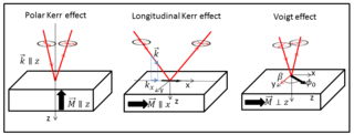
The Voigt effect is a magneto-optical phenomenon which rotates and elliptizes linearly polarised light sent into an optically active medium. The effect is named after the German scientist Woldemar Voigt who discovered it in vapors. Unlike many other magneto-optical effects such as the Kerr or Faraday effect which are linearly proportional to the magnetization, the Voigt effect is proportional to the square of the magnetization and can be seen experimentally at normal incidence. There are also other denominations for this effect, used interchangeably in the modern scientific literature: the Cotton–Mouton effect and magnetic-linear birefringence, with the latter reflecting the physical meaning of the effect.

<span class="mw-page-title-main">Jaynes–Cummings model</span> Model in quantum optics

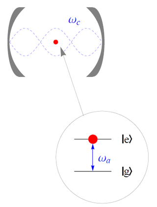
The Jaynes–Cummings model is a theoretical model in quantum optics. It describes the system of a two-level atom interacting with a quantized mode of an optical cavity, with or without the presence of light. It was originally developed to study the interaction of atoms with the quantized electromagnetic field in order to investigate the phenomena of spontaneous emission and absorption of photons in a cavity.

Sinusoidal plane-wave solutions are particular solutions to the electromagnetic wave equation.

Photon polarization is the quantum mechanical description of the classical polarized sinusoidal plane electromagnetic wave. An individual photon can be described as having right or left circular polarization, or a superposition of the two. Equivalently, a photon can be described as having horizontal or vertical linear polarization, or a superposition of the two.

In mathematics, the Schur orthogonality relations, which were proven by Issai Schur through Schur's lemma, express a central fact about representations of finite groups. They admit a generalization to the case of compact groups in general, and in particular compact Lie groups, such as the rotation group SO(3).

Acoustic streaming is a steady flow in a fluid driven by the absorption of high amplitude acoustic oscillations. This phenomenon can be observed near sound emitters, or in the standing waves within a Kundt's tube. Acoustic streaming was explained first by Lord Rayleigh in 1884. It is the less-known opposite of sound generation by a flow.

<span class="mw-page-title-main">Symmetry in quantum mechanics</span> Properties underlying modern physics

Symmetries in quantum mechanics describe features of spacetime and particles which are unchanged under some transformation, in the context of quantum mechanics, relativistic quantum mechanics and quantum field theory, and with applications in the mathematical formulation of the standard model and condensed matter physics. In general, symmetry in physics, invariance, and conservation laws, are fundamentally important constraints for formulating physical theories and models. In practice, they are powerful methods for solving problems and predicting what can happen. While conservation laws do not always give the answer to the problem directly, they form the correct constraints and the first steps to solving a multitude of problems.

References

  1. Gade, Kenneth (2016). "The Seven Ways to Find Heading" (PDF). The Journal of Navigation. Cambridge University Press. 69 (5): 955–970. doi:10.1017/S0373463316000096. S2CID   53587934.
  2. 1 2 3 4 Elliott-Laboratories (2003). The Anschutz Gyro-Compass and Gyroscope Engineering. Watchmaker. pp. 7–24. ISBN   978-1-929148-12-7. Archived from the original on 2017-03-04.
  3. 1 2 3 4 5 6 Time Inc. (Mar 15, 1943). "The gyroscope pilots ships & planes". Life. pp. 80–83. Archived from the original on 2017-02-27.
  4. 1 2 Safe Nav Watch. Edinburgh: Witherby Publishing Group. 2023. pp. 26–27. ISBN   9781914993466.
  5. 1 2 3 Galison, Peter (1987). How experiments end. University of Chicago Press. pp. 34–37. ISBN   978-0-226-27915-2. Archived from the original on 2012-03-02.
  6. "Archived copy" (PDF). Archived (PDF) from the original on 2015-06-29. Retrieved 2012-02-19.{{cite web}}: CS1 maint: archived copy as title (link) Standard 22 Anschütz Gyro Compass [sic] System: Gyro Compass [sic] Technology [sic] for over than [sic] 100 years
  7. Chambers of Commerce and Industry in Schleswig-Holstein Archived 2017-02-22 at the Wayback Machine Retrieved on February 22, 2017.
  8. 1 2 Gyrocompass, Auxiliary Gyrocompass, and Dead Reckoning Analyzing Indicator and Tracer Systems Archived 2013-06-01 at the Wayback Machine , San Francisco Maritime National Park Association.
  9. The Invention of Precision Navigational Instruments for Air and Sea Navigation Archived 2011-07-18 at the Wayback Machine , Weems & Plath.
  10. Collinson, R. P. G. (2003), Introduction to avionics systems, Springer, p. 293, ISBN   978-1-4020-7278-9, archived from the original on 2014-07-07
  11. NASA NASA Callback: Heading for Trouble Archived 2011-07-16 at the Wayback Machine , NASA Callback Safety Bulletin website, December 2005, No. 305. Retrieved August 29, 2010.
  12. Bowditch, Nathaniel. American Practical Navigator Archived 2017-03-07 at the Wayback Machine , Paradise Cay Publications, 2002, pp.93-94, ISBN   978-0-939837-54-0.
  13. Gyrocompass: Steaming Error Archived 2008-12-22 at the Wayback Machine , Navis. Accessed 15 December 2008.
  14. Seamanship Techniques:Shipboard and Marine Operations, D. J. House, Butterworth-Heinemann, 2004, p. 341

Bibliography