
A centripetal force is a force that makes a body follow a curved path. The direction of the centripetal force is always orthogonal to the motion of the body and towards the fixed point of the instantaneous center of curvature of the path. Isaac Newton described it as "a force by which bodies are drawn or impelled, or in any way tend, towards a point as to a centre". In the theory of Newtonian mechanics, gravity provides the centripetal force causing astronomical orbits.
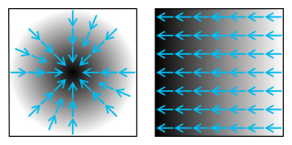
In vector calculus, the gradient of a scalar-valued differentiable function of several variables is the vector field whose value at a point gives the direction and the rate of fastest increase. The gradient transforms like a vector under change of basis of the space of variables of . If the gradient of a function is non-zero at a point , the direction of the gradient is the direction in which the function increases most quickly from , and the magnitude of the gradient is the rate of increase in that direction, the greatest absolute directional derivative. Further, a point where the gradient is the zero vector is known as a stationary point. The gradient thus plays a fundamental role in optimization theory, where it is used to maximize a function by gradient ascent. In coordinate-free terms, the gradient of a function may be defined by:
In mechanics and physics, simple harmonic motion is a special type of periodic motion an object experiences due to a restoring force whose magnitude is directly proportional to the distance of the object from an equilibrium position and acts towards the equilibrium position. It results in an oscillation that is described by a sinusoid which continues indefinitely.
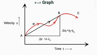
In physics, equations of motion are equations that describe the behavior of a physical system in terms of its motion as a function of time. More specifically, the equations of motion describe the behavior of a physical system as a set of mathematical functions in terms of dynamic variables. These variables are usually spatial coordinates and time, but may include momentum components. The most general choice are generalized coordinates which can be any convenient variables characteristic of the physical system. The functions are defined in a Euclidean space in classical mechanics, but are replaced by curved spaces in relativity. If the dynamics of a system is known, the equations are the solutions for the differential equations describing the motion of the dynamics.
In mathematics and science, a nonlinear system is a system in which the change of the output is not proportional to the change of the input. Nonlinear problems are of interest to engineers, biologists, physicists, mathematicians, and many other scientists since most systems are inherently nonlinear in nature. Nonlinear dynamical systems, describing changes in variables over time, may appear chaotic, unpredictable, or counterintuitive, contrasting with much simpler linear systems.
In the mathematical field of differential geometry, a metric tensor is an additional structure on a manifold M that allows defining distances and angles, just as the inner product on a Euclidean space allows defining distances and angles there. More precisely, a metric tensor at a point p of M is a bilinear form defined on the tangent space at p, and a metric tensor on M consists of a metric tensor at each point p of M that varies smoothly with p.
In the calculus of variations, a field of mathematical analysis, the functional derivative relates a change in a functional to a change in a function on which the functional depends.
The primitive equations are a set of nonlinear partial differential equations that are used to approximate global atmospheric flow and are used in most atmospheric models. They consist of three main sets of balance equations:
- A continuity equation: Representing the conservation of mass.
- Conservation of momentum: Consisting of a form of the Navier–Stokes equations that describe hydrodynamical flow on the surface of a sphere under the assumption that vertical motion is much smaller than horizontal motion (hydrostasis) and that the fluid layer depth is small compared to the radius of the sphere
- A thermal energy equation: Relating the overall temperature of the system to heat sources and sinks
In differential geometry, a one-form on a differentiable manifold is a smooth section of the cotangent bundle. Equivalently, a one-form on a manifold is a smooth mapping of the total space of the tangent bundle of to whose restriction to each fibre is a linear functional on the tangent space. Symbolically,
In mathematics, the covariant derivative is a way of specifying a derivative along tangent vectors of a manifold. Alternatively, the covariant derivative is a way of introducing and working with a connection on a manifold by means of a differential operator, to be contrasted with the approach given by a principal connection on the frame bundle – see affine connection. In the special case of a manifold isometrically embedded into a higher-dimensional Euclidean space, the covariant derivative can be viewed as the orthogonal projection of the Euclidean directional derivative onto the manifold's tangent space. In this case the Euclidean derivative is broken into two parts, the extrinsic normal component and the intrinsic covariant derivative component.

A vibration in a string is a wave. Resonance causes a vibrating string to produce a sound with constant frequency, i.e. constant pitch. If the length or tension of the string is correctly adjusted, the sound produced is a musical tone. Vibrating strings are the basis of string instruments such as guitars, cellos, and pianos.
In differential topology, the jet bundle is a certain construction that makes a new smooth fiber bundle out of a given smooth fiber bundle. It makes it possible to write differential equations on sections of a fiber bundle in an invariant form. Jets may also be seen as the coordinate free versions of Taylor expansions.
In mathematics, the Helmholtz equation is the eigenvalue problem for the Laplace operator. It corresponds to the linear partial differential equation
In fluid dynamics, dispersion of water waves generally refers to frequency dispersion, which means that waves of different wavelengths travel at different phase speeds. Water waves, in this context, are waves propagating on the water surface, with gravity and surface tension as the restoring forces. As a result, water with a free surface is generally considered to be a dispersive medium.
When studying and formulating Albert Einstein's theory of general relativity, various mathematical structures and techniques are utilized. The main tools used in this geometrical theory of gravitation are tensor fields defined on a Lorentzian manifold representing spacetime. This article is a general description of the mathematics of general relativity.

A pendulum is a body suspended from a fixed support so that it swings freely back and forth under the influence of gravity. When a pendulum is displaced sideways from its resting, equilibrium position, it is subject to a restoring force due to gravity that will accelerate it back toward the equilibrium position. When released, the restoring force acting on the pendulum's mass causes it to oscillate about the equilibrium position, swinging it back and forth. The mathematics of pendulums are in general quite complicated. Simplifying assumptions can be made, which in the case of a simple pendulum allow the equations of motion to be solved analytically for small-angle oscillations.
Miniaturizing components has always been a primary goal in the semiconductor industry because it cuts production cost and lets companies build smaller computers and other devices. Miniaturization, however, has increased dissipated power per unit area and made it a key limiting factor in integrated circuit performance. Temperature increase becomes relevant for relatively small-cross-sections wires, where it may affect normal semiconductor behavior. Besides, since the generation of heat is proportional to the frequency of operation for switching circuits, fast computers have larger heat generation than slow ones, an undesired effect for chips manufacturers. This article summaries physical concepts that describe the generation and conduction of heat in an integrated circuit, and presents numerical methods that model heat transfer from a macroscopic point of view.
In optics, the Fraunhofer diffraction equation is used to model the diffraction of waves when the diffraction pattern is viewed at a long distance from the diffracting object, and also when it is viewed at the focal plane of an imaging lens.

In continuum mechanics, Whitham's averaged Lagrangian method – or in short Whitham's method – is used to study the Lagrangian dynamics of slowly-varying wave trains in an inhomogeneous (moving) medium. The method is applicable to both linear and non-linear systems. As a direct consequence of the averaging used in the method, wave action is a conserved property of the wave motion. In contrast, the wave energy is not necessarily conserved, due to the exchange of energy with the mean motion. However the total energy, the sum of the energies in the wave motion and the mean motion, will be conserved for a time-invariant Lagrangian. Further, the averaged Lagrangian has a strong relation to the dispersion relation of the system.

In fluid dynamics, Green's law, named for 19th-century British mathematician George Green, is a conservation law describing the evolution of non-breaking, surface gravity waves propagating in shallow water of gradually varying depth and width. In its simplest form, for wavefronts and depth contours parallel to each other, it states:


