In mathematics, the tangent space of a manifold is a generalization of tangent lines to curves in two-dimensional space and tangent planes to surfaces in three-dimensional space in higher dimensions. In the context of physics the tangent space to a manifold at a point can be viewed as the space of possible velocities for a particle moving on the manifold.
In probability theory, the central limit theorem (CLT) states that, under appropriate conditions, the distribution of a normalized version of the sample mean converges to a standard normal distribution. This holds even if the original variables themselves are not normally distributed. There are several versions of the CLT, each applying in the context of different conditions.

In complex analysis, the residue theorem, sometimes called Cauchy's residue theorem, is a powerful tool to evaluate line integrals of analytic functions over closed curves; it can often be used to compute real integrals and infinite series as well. It generalizes the Cauchy integral theorem and Cauchy's integral formula. The residue theorem should not be confused with special cases of the generalized Stokes' theorem; however, the latter can be used as an ingredient of its proof.
In vector calculus, Green's theorem relates a line integral around a simple closed curve C to a double integral over the plane region D bounded by C. It is the two-dimensional special case of Stokes' theorem.

In mathematics, a Green's function is the impulse response of an inhomogeneous linear differential operator defined on a domain with specified initial conditions or boundary conditions.
In mathematics, the Mellin transform is an integral transform that may be regarded as the multiplicative version of the two-sided Laplace transform. This integral transform is closely connected to the theory of Dirichlet series, and is often used in number theory, mathematical statistics, and the theory of asymptotic expansions; it is closely related to the Laplace transform and the Fourier transform, and the theory of the gamma function and allied special functions.

In mathematics, theta functions are special functions of several complex variables. They show up in many topics, including Abelian varieties, moduli spaces, quadratic forms, and solitons. As Grassmann algebras, they appear in quantum field theory.
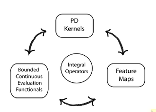
In functional analysis, a reproducing kernel Hilbert space (RKHS) is a Hilbert space of functions in which point evaluation is a continuous linear functional. Roughly speaking, this means that if two functions and in the RKHS are close in norm, i.e., is small, then and are also pointwise close, i.e., is small for all . The converse does not need to be true. Informally, this can be shown by looking at the supremum norm: the sequence of functions converges pointwise, but does not converge uniformly i.e. does not converge with respect to the supremum norm.
In mathematics, the Lerch zeta function, sometimes called the Hurwitz–Lerch zeta function, is a special function that generalizes the Hurwitz zeta function and the polylogarithm. It is named after Czech mathematician Mathias Lerch, who published a paper about the function in 1887.

In quantum field theory, the Lehmann–Symanzik–Zimmermann (LSZ) reduction formula is a method to calculate S-matrix elements from the time-ordered correlation functions of a quantum field theory. It is a step of the path that starts from the Lagrangian of some quantum field theory and leads to prediction of measurable quantities. It is named after the three German physicists Harry Lehmann, Kurt Symanzik and Wolfhart Zimmermann.

Arc length is the distance between two points along a section of a curve.
In Bayesian probability, the Jeffreys prior, named after Sir Harold Jeffreys, is a non-informative prior distribution for a parameter space; its density function is proportional to the square root of the determinant of the Fisher information matrix:
In mathematics, the explicit formulae for L-functions are relations between sums over the complex number zeroes of an L-function and sums over prime powers, introduced by Riemann (1859) for the Riemann zeta function. Such explicit formulae have been applied also to questions on bounding the discriminant of an algebraic number field, and the conductor of a number field.

In probability theory and statistics, the characteristic function of any real-valued random variable completely defines its probability distribution. If a random variable admits a probability density function, then the characteristic function is the Fourier transform of the probability density function. Thus it provides an alternative route to analytical results compared with working directly with probability density functions or cumulative distribution functions. There are particularly simple results for the characteristic functions of distributions defined by the weighted sums of random variables.
In mathematics and economics, transportation theory or transport theory is a name given to the study of optimal transportation and allocation of resources. The problem was formalized by the French mathematician Gaspard Monge in 1781.
A ratio distribution is a probability distribution constructed as the distribution of the ratio of random variables having two other known distributions. Given two random variables X and Y, the distribution of the random variable Z that is formed as the ratio Z = X/Y is a ratio distribution.

In geometry, a ball is a region in a space comprising all points within a fixed distance, called the radius, from a given point; that is, it is the region enclosed by a sphere or hypersphere. An n-ball is a ball in an n-dimensional Euclidean space. The volume of a n-ball is the Lebesgue measure of this ball, which generalizes to any dimension the usual volume of a ball in 3-dimensional space. The volume of a n-ball of radius R is where is the volume of the unit n-ball, the n-ball of radius 1.
In mathematics, Watson's lemma, proved by G. N. Watson, has significant application within the theory on the asymptotic behavior of integrals.
Lagrangian field theory is a formalism in classical field theory. It is the field-theoretic analogue of Lagrangian mechanics. Lagrangian mechanics is used to analyze the motion of a system of discrete particles each with a finite number of degrees of freedom. Lagrangian field theory applies to continua and fields, which have an infinite number of degrees of freedom.
In representation theory of mathematics, the Waldspurger formula relates the special values of two L-functions of two related admissible irreducible representations. Let k be the base field, f be an automorphic form over k, π be the representation associated via the Jacquet–Langlands correspondence with f. Goro Shimura (1976) proved this formula, when and f is a cusp form; Günter Harder made the same discovery at the same time in an unpublished paper. Marie-France Vignéras (1980) proved this formula, when and f is a newform. Jean-Loup Waldspurger, for whom the formula is named, reproved and generalized the result of Vignéras in 1985 via a totally different method which was widely used thereafter by mathematicians to prove similar formulas.


