Integral as area between two curves.Double integral as volume under a surface z = 10 − (x − y/8). The rectangular region at the bottom of the body is the domain of integration, while the surface is the graph of the two-variable function to be integrated.
Integrals of a function of two variables over a region in (the real-number plane) are called double integrals, and integrals of a function of three variables over a region in (real-number 3D space) are called triple integrals.[1] For multiple integrals of a single-variable function, see the Cauchy formula for repeated integration.
Introduction
Just as the definite integral of a positive function of one variable represents the area of the region between the graph of the function and the x-axis, the double integral of a positive function of two variables represents the volume of the region between the surface defined by the function (on the three-dimensional Cartesian plane where z = f(x, y)) and the plane which contains its domain.[1] If there are more variables, a multiple integral will yield hypervolumes of multidimensional functions.
Multiple integration of a function in n variables: f(x1, x2, ..., xn) over a domain D is most commonly represented by nested integral signs in the reverse order of execution (the leftmost integral sign is computed last), followed by the function and integrand arguments in proper order (the integral with respect to the rightmost argument is computed last). The domain of integration is either represented symbolically for every argument over each integral sign, or is abbreviated by a variable at the rightmost integral sign:[2]
Since the concept of an antiderivative is only defined for functions of a single real variable, the usual definition of the indefinite integral does not immediately extend to the multiple integral.
Mathematical definition
For n > 1, consider a so-called "half-open" n-dimensional hyperrectangular domain T, defined as
.
Partition each interval [aj, bj) into a finite family Ij of non-overlapping subintervals ijα, with each subinterval closed at the left end, and open at the right end.
Then the finite family of subrectangles C given by
is a partition of T; that is, the subrectangles Ck are non-overlapping and their union is T.
Let f: T → R be a function defined on T. Consider a partition C of T as defined above, such that C is a family of m subrectangles Cm and
We can approximate the total (n + 1)-dimensional volume bounded below by the n-dimensional hyperrectangle T and above by the n-dimensional graph of f with the following Riemann sum:
where Pk is a point in Ck and m(Ck) is the product of the lengths of the intervals whose Cartesian product is Ck, also known as the measure of Ck.
The diameter of a subrectangle Ck is the largest of the lengths of the intervals whose Cartesian product is Ck. The diameter of a given partition of T is defined as the largest of the diameters of the subrectangles in the partition. Intuitively, as the diameter of the partition C is restricted smaller and smaller, the number of subrectangles m gets larger, and the measure m(Ck) of each subrectangle grows smaller. The function f is said to be Riemann integrable if the limit
exists, where the limit is taken over all possible partitions of T of diameter at most δ.[3]
If f is Riemann integrable, S is called the Riemann integral of f over T and is denoted
.
Frequently this notation is abbreviated as
.
where x represents the n-tuple (x1, ..., xn) and dnx is the n-dimensional volume differential.
The Riemann integral of a function defined over an arbitrary bounded n-dimensional set can be defined by extending that function to a function defined over a half-open rectangle whose values are zero outside the domain of the original function. Then the integral of the original function over the original domain is defined to be the integral of the extended function over its rectangular domain, if it exists.
In what follows the Riemann integral in n dimensions will be called the multiple integral.
Properties
Multiple integrals have many properties common to those of integrals of functions of one variable (linearity, commutativity, monotonicity, and so on). One important property of multiple integrals is that the value of an integral is independent of the order of integrands under certain conditions. This property is popularly known as Fubini's theorem.[4]
Particular cases
In the case of , the integral
is the double integral of f on T, and if the integral
is the triple integral of f on T.
Notice that, by convention, the double integral has two integral signs, and the triple integral has three; this is a notational convention which is convenient when computing a multiple integral as an iterated integral, as shown later in this article.
Methods of integration
The resolution of problems with multiple integrals consists, in most cases, of finding a way to reduce the multiple integral to an iterated integral, a series of integrals of one variable, each being directly solvable. For continuous functions, this is justified by Fubini's theorem. Sometimes, it is possible to obtain the result of the integration by direct examination without any calculations.
The following are some simple methods of integration:[1]
Integrating constant functions
When the integrand is a constant functionc, the integral is equal to the product of c and the measure of the domain of integration. If c = 1 and the domain is a subregion of R2, the integral gives the area of the region, while if the domain is a subregion of R3, the integral gives the volume of the region.
Example. Let f(x, y) = 2 and
,
in which case
,
since by definition we have:
.
Use of symmetry
When the domain of integration is symmetric about the origin with respect to at least one of the variables of integration and the integrand is odd with respect to this variable, the integral is equal to zero, as the integrals over the two halves of the domain have the same absolute value but opposite signs. When the integrand is even with respect to this variable, the integral is equal to twice the integral over one half of the domain, as the integrals over the two halves of the domain are equal.
Example 1. Consider the function f(x,y) = 2 sin(x) − 3y3 + 5 integrated over the domain
,
a disc with radius1 centered at the origin with the boundary included.
Using the linearity property, the integral can be decomposed into three pieces:
.
The function 2 sin(x) is an odd function in the variable x and the disc T is symmetric with respect to the y-axis, so the value of the first integral is 0. Similarly, the function 3y3 is an odd function of y, and T is symmetric with respect to the x-axis, and so the only contribution to the final result is that of the third integral. Therefore the original integral is equal to the area of the disk times 5, or 5π.
Example 2. Consider the function f(x, y, z) = x exp(y2 + z2) and as integration region the ball with radius 2 centered at the origin,
.
The "ball" is symmetric about all three axes, but it is sufficient to integrate with respect to x-axis to show that the integral is 0, because the function is an odd function of that variable.
This method is applicable to any domain D for which:
The projection of D onto either the x-axis or the y-axis is bounded by the two values, a and b
Any line perpendicular to this axis that passes between these two values intersects the domain in an interval whose endpoints are given by the graphs of two functions, α and β
Such a domain will be here called a normal domain. Elsewhere in the literature, normal domains are sometimes called type I or type II domains, depending on which axis the domain is fibred over. In all cases, the function to be integrated must be Riemann integrable on the domain, which is true (for instance) if the function is continuous.
x-axis
If the domain D is normal with respect to the x-axis, and f: D → R is a continuous function; then α(x) and β(x) (both of which are defined on the interval [a, b]) are the two functions that determine D. Then, by Fubini's theorem:[5]
.
y-axis
If D is normal with respect to the y-axis and f: D → R is a continuous function; then α(y) and β(y) (both of which are defined on the interval [a, b]) are the two functions that determine D. Again, by Fubini's theorem:
.
Normal domains on R3
If T is a domain that is normal with respect to the xy-plane and determined by the functions α(x, y) and β(x, y), then
.
This definition is the same for the other five normality cases on R3. It can be generalized in a straightforward way to domains in Rn.
The limits of integration are often not easily interchangeable (without normality or with complex formulae to integrate). One makes a change of variables to rewrite the integral in a more "comfortable" region, which can be described in simpler formulae. To do so, the function must be adapted to the new coordinates.
Example 1a. The function is f(x, y) = (x − 1)2 + √y; if one adopts the substitution u = x − 1, v = y therefore x = u + 1, y = v one obtains the new function f2(u, v) = (u)2 + √v.
Similarly for the domain because it is delimited by the original variables that were transformed before (x and y in example)
The differentials dx and dy transform via the absolute value of the determinant of the Jacobian matrix containing the partial derivatives of the transformations regarding the new variable (consider, as an example, the differential transformation in polar coordinates)
There exist three main "kinds" of changes of variable (one in R2, two in R3); however, more general substitutions can be made using the same principle.
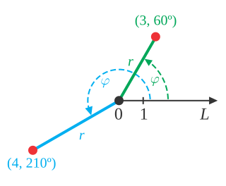
Transformation from cartesian to polar coordinates.
In R2 if the domain has a circular symmetry and the function has some particular characteristics one can apply the transformation to polar coordinates (see the example in the picture) which means that the generic points P(x, y) in Cartesian coordinates switch to their respective points in polar coordinates. That allows one to change the shape of the domain and simplify the operations.
The fundamental relation to make the transformation is the following:
.
Example 2a. The function is f(x, y) = x + y and applying the transformation one obtains
.
Example 2b. The function is f(x, y) = x2 + y2, in this case one has:
The transformation of the domain is made by defining the radius' crown length and the amplitude of the described angle to define the ρ, φ intervals starting from x, y.
Example of a domain transformation from cartesian to polar.
Example 2c. The domain is D = {x2 + y2 ≤ 4}, that is a circumference of radius 2; it's evident that the covered angle is the circle angle, so φ varies from 0 to 2π, while the crown radius varies from 0 to 2 (the crown with the inside radius null is just a circle).
Example 2d. The domain is D = {x2 + y2 ≤ 9, x2 + y2 ≥ 4, y ≥ 0}, that is the circular crown in the positive y half-plane (please see the picture in the example); φ describes a plane angle while ρ varies from 2 to 3. Therefore the transformed domain will be the following rectangle:
which has been obtained by inserting the partial derivatives of x = ρ cos(φ), y = ρ sin(φ) in the first column respect to ρ and in the second respect to φ, so the dx dy differentials in this transformation become ρ dρ dφ.
Once the function is transformed and the domain evaluated, it is possible to define the formula for the change of variables in polar coordinates:
.
φ is valid in the [0, 2π] interval while ρ, which is a measure of a length, can only have positive values.
Example 2e. The function is f(x, y) = x and the domain is the same as in Example 2d. From the previous analysis of D we know the intervals of ρ (from 2 to 3) and of φ (from 0 to π). Now we change the function:
.
Finally let's apply the integration formula:
.
Once the intervals are known, you have
.
Cylindrical coordinates
Cylindrical coordinates.
In R3 the integration on domains with a circular base can be made by the passage to cylindrical coordinates; the transformation of the function is made by the following relation:
The domain transformation can be graphically attained, because only the shape of the base varies, while the height follows the shape of the starting region.
Example 3a. The region is D = {x2 + y2 ≤ 9, x2 + y2 ≥ 4, 0 ≤ z ≤ 5} (that is the "tube" whose base is the circular crown of Example 2d and whose height is 5); if the transformation is applied, this region is obtained:
(that is, the parallelepiped whose base is similar to the rectangle in Example 2d and whose height is 5).
Because the z component is unvaried during the transformation, the dx dy dz differentials vary as in the passage to polar coordinates: therefore, they become ρ dρ dφ dz.
Finally, it is possible to apply the final formula to cylindrical coordinates:
.
This method is convenient in case of cylindrical or conical domains or in regions where it is easy to individuate the z interval and even transform the circular base and the function.
Example 3b. The function is f(x, y, z) = x2 + y2 + z and as integration domain this cylinder: D = {x2 + y2 ≤ 9, −5 ≤ z ≤ 5}. The transformation of D in cylindrical coordinates is the following:
.
while the function becomes
.
Finally one can apply the integration formula:
;
developing the formula you have
.
Spherical coordinates
Spherical coordinates.
In R3 some domains have a spherical symmetry, so it's possible to specify the coordinates of every point of the integration region by two angles and one distance. It's possible to use therefore the passage to spherical coordinates; the function is transformed by this relation:
.
Points on the z-axis do not have a precise characterization in spherical coordinates, so θ can vary between 0 and 2π.
The better integration domain for this passage is the sphere.
Example 4a. The domain is D = x2 + y2 + z2 ≤ 16 (sphere with radius 4 and center at the origin); applying the transformation you get the region
.
The Jacobian determinant of this transformation is the following:
.
The dx dy dz differentials therefore are transformed to ρ2 sin(φ) dρdθdφ.
This yields the final integration formula:
.
It is better to use this method in case of spherical domains and in case of functions that can be easily simplified by the first fundamental relation of trigonometry extended to R3 (see Example 4b); in other cases it can be better to use cylindrical coordinates (see Example 4c).
.
The extra ρ2 and sin φ come from the Jacobian.
In the following examples the roles of φ and θ have been reversed.
Example 4b.D is the same region as in Example 4a and f(x, y, z) = x2 + y2 + z2 is the function to integrate. Its transformation is very easy:
,
while we know the intervals of the transformed region T from D:
.
We therefore apply the integration formula:
,
and, developing, we get
.
Example 4c. The domain D is the ball with center at the origin and radius 3a,
,
and f(x, y, z) = x2 + y2 is the function to integrate.
Looking at the domain, it seems convenient to adopt the passage to spherical coordinates, in fact, the intervals of the variables that delimit the new T region are:
.
However, applying the transformation, we get
.
Applying the formula for integration we obtain:
,
which can be solved by turning it into an iterated integral..
,
,
.
Collecting all parts,
.
Alternatively, this problem can be solved by using the passage to cylindrical coordinates. The new T intervals are
;
the z interval has been obtained by dividing the ball into two hemispheres simply by solving the inequality from the formula of D (and then directly transforming x2 + y2 into ρ2). The new function is simply ρ2. Applying the integration formula
.
Then we get:
Thanks to the passage to cylindrical coordinates it was possible to reduce the triple integral to an easier one-variable integral.
Let us assume that we wish to integrate a multivariable function f over a region A:
.
From this we formulate the iterated integral
.
The inner integral is performed first, integrating with respect to x and taking y as a constant, as it is not the variable of integration. The result of this integral, which is a function depending only on y, is then integrated with respect to y.
We then integrate the result with respect to y.
In cases where the double integral of the absolute value of the function is finite, the order of integration is interchangeable, that is, integrating with respect to x first and integrating with respect to y first produce the same result. That is Fubini's theorem. For example, doing the previous calculation with order reversed gives the same result:
Double integral over a normal domain
Example: double integral over the normal region D
Consider the region (please see the graphic in the example):
.
Calculate
.
This domain is normal with respect to both the x- and y-axes. To apply the formulae it is required to find the functions that determine D and the intervals over which these functions are defined. In this case the two functions are:
while the interval is given by the intersections of the functions with x=0, so the interval is [a,b] = [0,1] (normality has been chosen with respect to the x-axis for a better visual understanding).
It is now possible to apply the formula:
(at first the second integral is calculated considering x as a constant). The remaining operations consist of applying the basic techniques of integration:
.
If we choose normality with respect to the y-axis we could calculate
.
and obtain the same value.
Example of domain in R that is normal with respect to the xy-plane.
Calculating volume
Using the methods previously described, it is possible to calculate the volumes of some common solids.
Cylinder: The volume of a cylinder with height h and circular base of radius R can be calculated by integrating the constant function h over the circular base, using polar coordinates.
This is in agreement with the formula for the volume of a prism
.
Sphere: The volume of a sphere with radius R can be calculated by integrating the constant function 1 over the sphere, using spherical coordinates.
Tetrahedron (triangular pyramid or 3-simplex): The volume of a tetrahedron with its apex at the origin and edges of length ℓ along the x-, y- and z-axes can be calculated by integrating the constant function 1 over the tetrahedron.
This is in agreement with the formula for the volume of a pyramid.
.
Example of an improper domain.
Multiple improper integral
In case of unbounded domains or functions not bounded near the boundary of the domain, we have to introduce the double improper integral or the triple improper integral.
If the integral is not absolutely convergent, care is needed not to confuse the concepts of multiple integral and iterated integral, especially since the same notation is often used for either concept. The notation
means, in some cases, an iterated integral rather than a true double integral. In an iterated integral, the outer integral
is the integral with respect to x of the following function of x:
.
A double integral, on the other hand, is defined with respect to area in the xy-plane. If the double integral exists, then it is equal to each of the two iterated integrals (either "dy dx" or "dx dy") and one often computes it by computing either of the iterated integrals. But sometimes the two iterated integrals exist when the double integral does not, and in some such cases the two iterated integrals are different numbers, i.e., one has
On the other hand, some conditions ensure that the two iterated integrals are equal even though the double integral need not exist. By the Fichtenholz–Lichtenstein theorem, if f is bounded on [0, 1] × [0, 1] and both iterated integrals exist, then they are equal. Moreover, existence of the inner integrals ensures existence of the outer integrals.[6][7][8] The double integral need not exist in this case even as Lebesgue integral, according to Sierpiński.[9]
The notation
may be used if one wishes to be emphatic about intending a double integral rather than an iterated integral.
Triple integral was demonstrated by Fubini's theorem.[10] Drichlet theorem and Liouville 's extension theorem on Triple integral.
Some practical applications
Quite generally, just as in one variable, one can use the multiple integral to find the average of a function over a given set. Given a set D ⊆ Rn and an integrable function f over D, the average value of f over its domain is given by
Additionally, multiple integrals are used in many applications in physics. The examples below also show some variations in the notation.
In mechanics, the moment of inertia is calculated as the volume integral (triple integral) of the density weighed with the square of the distance from the axis:
If there is a continuous function ρ(x) representing the density of the distribution at x, so that dm(x) = ρ(x)d3x, where d3x is the Euclidean volume element, then the gravitational potential is
.
In electromagnetism, Maxwell's equations can be written using multiple integrals to calculate the total magnetic and electric fields.[12] In the following example, the electric field produced by a distribution of charges given by the volume charge densityρ( r→ ) is obtained by a triple integral of a vector function:
.
This can also be written as an integral with respect to a signed measure representing the charge distribution.
See also
Main analysis theorems that relate multiple integrals:
In mathematics, the polar coordinate system is a two-dimensional coordinate system in which each point on a plane is determined by a distance from a reference point and an angle from a reference direction. The reference point is called the pole, and the ray from the pole in the reference direction is the polar axis. The distance from the pole is called the radial coordinate, radial distance or simply radius, and the angle is called the angular coordinate, polar angle, or azimuth. Angles in polar notation are generally expressed in either degrees or radians.
In mathematics and physics, Laplace's equation is a second-order partial differential equation named after Pierre-Simon Laplace, who first studied its properties. This is often written as
The Navier–Stokes equations are partial differential equations which describe the motion of viscous fluid substances. They were named after French engineer and physicist Claude-Louis Navier and the Irish physicist and mathematician George Gabriel Stokes. They were developed over several decades of progressively building the theories, from 1822 (Navier) to 1842–1850 (Stokes).
In vector calculus, the Jacobian matrix of a vector-valued function of several variables is the matrix of all its first-order partial derivatives. When this matrix is square, that is, when the function takes the same number of variables as input as the number of vector components of its output, its determinant is referred to as the Jacobian determinant. Both the matrix and the determinant are often referred to simply as the Jacobian in literature.
In geometry, a solid of revolution is a solid figure obtained by rotating a plane figure around some straight line, which may not intersect the generatrix. The surface created by this revolution and which bounds the solid is the surface of revolution.
A surface of revolution is a surface in Euclidean space created by rotating a curve one full revolution around an axis of rotation . The volume bounded by the surface created by this revolution is the solid of revolution.
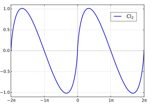
In mathematics, the Clausen function, introduced by Thomas Clausen, is a transcendental, special function of a single variable. It can variously be expressed in the form of a definite integral, a trigonometric series, and various other forms. It is intimately connected with the polylogarithm, inverse tangent integral, polygamma function, Riemann zeta function, Dirichlet eta function, and Dirichlet beta function.
In probability theory, the Borel–Kolmogorov paradox is a paradox relating to conditional probability with respect to an event of probability zero. It is named after Émile Borel and Andrey Kolmogorov.
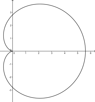
In geometry, a cardioid is a plane curve traced by a point on the perimeter of a circle that is rolling around a fixed circle of the same radius. It can also be defined as an epicycloid having a single cusp. It is also a type of sinusoidal spiral, and an inverse curve of the parabola with the focus as the center of inversion. A cardioid can also be defined as the set of points of reflections of a fixed point on a circle through all tangents to the circle.
This is a list of some vector calculus formulae for working with common curvilinear coordinate systems.
In mathematics, a volume integral (∭) is an integral over a 3-dimensional domain; that is, it is a special case of multiple integrals. Volume integrals are especially important in physics for many applications, for example, to calculate flux densities, or to calculate mass from a corresponding density function.
In calculus, the Leibniz integral rule for differentiation under the integral sign states that for an integral of the form
A ratio distribution is a probability distribution constructed as the distribution of the ratio of random variables having two other known distributions. Given two random variables X and Y, the distribution of the random variable Z that is formed as the ratio Z = X/Y is a ratio distribution.
In mathematics, vector spherical harmonics (VSH) are an extension of the scalar spherical harmonics for use with vector fields. The components of the VSH are complex-valued functions expressed in the spherical coordinate basis vectors.
In mathematics, the spectral theory of ordinary differential equations is the part of spectral theory concerned with the determination of the spectrum and eigenfunction expansion associated with a linear ordinary differential equation. In his dissertation, Hermann Weyl generalized the classical Sturm–Liouville theory on a finite closed interval to second order differential operators with singularities at the endpoints of the interval, possibly semi-infinite or infinite. Unlike the classical case, the spectrum may no longer consist of just a countable set of eigenvalues, but may also contain a continuous part. In this case the eigenfunction expansion involves an integral over the continuous part with respect to a spectral measure, given by the Titchmarsh–Kodaira formula. The theory was put in its final simplified form for singular differential equations of even degree by Kodaira and others, using von Neumann's spectral theorem. It has had important applications in quantum mechanics, operator theory and harmonic analysis on semisimple Lie groups.
A product distribution is a probability distribution constructed as the distribution of the product of random variables having two other known distributions. Given two statistically independent random variables X and Y, the distribution of the random variable Z that is formed as the product is a product distribution.
In geometry, a spherical sector, also known as a spherical cone, is a portion of a sphere or of a ball defined by a conical boundary with apex at the center of the sphere. It can be described as the union of a spherical cap and the cone formed by the center of the sphere and the base of the cap. It is the three-dimensional analogue of the sector of a circle.
In optics, the Fraunhofer diffraction equation is used to model the diffraction of waves when the diffraction pattern is viewed at a long distance from the diffracting object, and also when it is viewed at the focal plane of an imaging lens.
In mathematics, singular integral operators of convolution type are the singular integral operators that arise on Rn and Tn through convolution by distributions; equivalently they are the singular integral operators that commute with translations. The classical examples in harmonic analysis are the harmonic conjugation operator on the circle, the Hilbert transform on the circle and the real line, the Beurling transform in the complex plane and the Riesz transforms in Euclidean space. The continuity of these operators on L2 is evident because the Fourier transform converts them into multiplication operators. Continuity on Lp spaces was first established by Marcel Riesz. The classical techniques include the use of Poisson integrals, interpolation theory and the Hardy–Littlewood maximal function. For more general operators, fundamental new techniques, introduced by Alberto Calderón and Antoni Zygmund in 1952, were developed by a number of authors to give general criteria for continuity on Lp spaces. This article explains the theory for the classical operators and sketches the subsequent general theory.
This page is based on this Wikipedia article Text is available under the CC BY-SA 4.0 license; additional terms may apply. Images, videos and audio are available under their respective licenses.