provided that the limit exists for all , where the limit is taken for scalar . This is similar to the usual definition of a directional derivative but extends it to functions that are not necessarily scalar-valued.
Next, choose a set of basis vectors and consider the operators, denoted , that perform directional derivatives in the directions of :
where the geometric product is applied after the directional derivative. More verbosely:
This operator is independent of the choice of frame, and can thus be used to define what in geometric calculus is called the vector derivative:
This is similar to the usual definition of the gradient, but it, too, extends to functions that are not necessarily scalar-valued.
The directional derivative is linear regarding its direction, that is:
From this follows that the directional derivative is the inner product of its direction by the vector derivative. All needs to be observed is that the direction can be written , so that:
For this reason, is often noted .
The standard order of operations for the vector derivative is that it acts only on the function closest to its immediate right. Given two functions and , then for example we have
Product rule
Although the partial derivative exhibits a product rule, the vector derivative only partially inherits this property. Consider two functions and :
Since the geometric product is not commutative with in general, we need a new notation to proceed. A solution is to adopt the overdot notation, in which the scope of a vector derivative with an overdot is the multivector-valued function sharing the same overdot. In this case, if we define
then the product rule for the vector derivative is
Interior and exterior derivative
Let be an -grade multivector. Then we can define an additional pair of operators, the interior and exterior derivatives,
In particular, if is grade 1 (vector-valued function), then we can write
Unlike the vector derivative, neither the interior derivative operator nor the exterior derivative operator is invertible.
Multivector derivative
The derivative with respect to a vector as discussed above can be generalized to a derivative with respect to a general multivector, called the multivector derivative.
Let be a multivector-valued function of a multivector. The directional derivative of with respect to in the direction , where and are multivectors, is defined as
where is the scalar product. With a vector basis and the corresponding dual basis, the multivector derivative is defined in terms of the directional derivative as[2]
This equation is just expressing in terms of components in a reciprocal basis of blades, as discussed in the article section Geometric algebra#Dual basis.
A key property of the multivector derivative is that
where is the projection of onto the grades contained in .
Let be a set of basis vectors that span an -dimensional vector space. From geometric algebra, we interpret the pseudoscalar to be the signed volume of the -parallelotope subtended by these basis vectors. If the basis vectors are orthonormal, then this is the unit pseudoscalar.
More generally, we may restrict ourselves to a subset of of the basis vectors, where , to treat the length, area, or other general -volume of a subspace in the overall -dimensional vector space. We denote these selected basis vectors by . A general -volume of the -parallelotope subtended by these basis vectors is the grade multivector .
Even more generally, we may consider a new set of vectors proportional to the basis vectors, where each of the is a component that scales one of the basis vectors. We are free to choose components as infinitesimally small as we wish as long as they remain nonzero. Since the outer product of these terms can be interpreted as a -volume, a natural way to define a measure is
The measure is therefore always proportional to the unit pseudoscalar of a -dimensional subspace of the vector space. Compare the Riemannian volume form in the theory of differential forms. The integral is taken with respect to this measure:
More formally, consider some directed volume of the subspace. We may divide this volume into a sum of simplices. Let be the coordinates of the vertices. At each vertex we assign a measure as the average measure of the simplices sharing the vertex. Then the integral of with respect to over this volume is obtained in the limit of finer partitioning of the volume into smaller simplices:
Fundamental theorem of geometric calculus
The reason for defining the vector derivative and integral as above is that they allow a strong generalization of Stokes' theorem. Let be a multivector-valued function of -grade input and general position , linear in its first argument. Then the fundamental theorem of geometric calculus relates the integral of a derivative over the volume to the integral over its boundary:
As an example, let for a vector-valued function and a ()-grade multivector . We find that
A sufficiently smooth -surface in an -dimensional space is deemed a manifold. To each point on the manifold, we may attach a -blade that is tangent to the manifold. Locally, acts as a pseudoscalar of the -dimensional space. This blade defines a projection of vectors onto the manifold:
Just as the vector derivative is defined over the entire -dimensional space, we may wish to define an intrinsic derivative, locally defined on the manifold:
(Note: The right hand side of the above may not lie in the tangent space to the manifold. Therefore, it is not the same as , which necessarily does lie in the tangent space.)
If is a vector tangent to the manifold, then indeed both the vector derivative and intrinsic derivative give the same directional derivative:
Although this operation is perfectly valid, it is not always useful because itself is not necessarily on the manifold. Therefore, we define the covariant derivative to be the forced projection of the intrinsic derivative back onto the manifold:
Since any general multivector can be expressed as a sum of a projection and a rejection, in this case
we introduce a new function, the shape tensor, which satisfies
where is the commutator product. In a local coordinate basis spanning the tangent surface, the shape tensor is given by
Importantly, on a general manifold, the covariant derivative does not commute. In particular, the commutator is related to the shape tensor by
Clearly the term is of interest. However it, like the intrinsic derivative, is not necessarily on the manifold. Therefore, we can define the Riemann tensor to be the projection back onto the manifold:
Lastly, if is of grade , then we can define interior and exterior covariant derivatives as
We can alternatively introduce a -grade multivector as
and a measure
Apart from a subtle difference in meaning for the exterior product with respect to differential forms versus the exterior product with respect to vectors (in the former the increments are covectors, whereas in the latter they represent scalars), we see the correspondences of the differential form
embed the theory of differential forms within geometric calculus.
History
Following is a diagram summarizing the history of geometric calculus.
History of geometric calculus.
References and further reading
↑ David Hestenes, Garrett Sobczyk: Clifford Algebra to Geometric Calculus, a Unified Language for mathematics and Physics (Dordrecht/Boston:G.Reidel Publ.Co., 1984, ISBN90-277-2561-6
↑ Doran, Chris; Lasenby, Anthony (2007). Geometric Algebra for Physicists. Cambridge University press. p.395. ISBN978-0-521-71595-9.
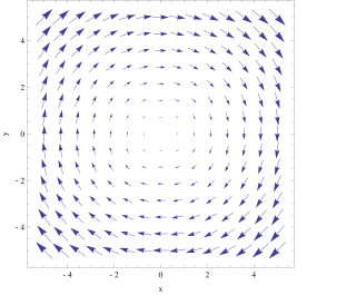
In vector calculus, the curl, also known as rotor, is a vector operator that describes the infinitesimal circulation of a vector field in three-dimensional Euclidean space. The curl at a point in the field is represented by a vector whose length and direction denote the magnitude and axis of the maximum circulation. The curl of a field is formally defined as the circulation density at each point of the field.
In vector calculus, divergence is a vector operator that operates on a vector field, producing a scalar field giving the quantity of the vector field's source at each point. More technically, the divergence represents the volume density of the outward flux of a vector field from an infinitesimal volume around a given point.
In mathematics, a geometric algebra is an extension of elementary algebra to work with geometrical objects such as vectors. Geometric algebra is built out of two fundamental operations, addition and the geometric product. Multiplication of vectors results in higher-dimensional objects called multivectors. Compared to other formalisms for manipulating geometric objects, geometric algebra is noteworthy for supporting vector division and addition of objects of different dimensions.
On a differentiable manifold, the exterior derivative extends the concept of the differential of a function to differential forms of higher degree. The exterior derivative was first described in its current form by Élie Cartan in 1899. The resulting calculus, known as exterior calculus, allows for a natural, metric-independent generalization of Stokes' theorem, Gauss's theorem, and Green's theorem from vector calculus.
In mathematics, differential forms provide a unified approach to define integrands over curves, surfaces, solids, and higher-dimensional manifolds. The modern notion of differential forms was pioneered by Élie Cartan. It has many applications, especially in geometry, topology and physics.
In mathematics, a differential operator is an operator defined as a function of the differentiation operator. It is helpful, as a matter of notation first, to consider differentiation as an abstract operation that accepts a function and returns another function.
In differential geometry, the Lie derivative, named after Sophus Lie by Władysław Ślebodziński, evaluates the change of a tensor field, along the flow defined by another vector field. This change is coordinate invariant and therefore the Lie derivative is defined on any differentiable manifold.
In mathematics, the Hodge star operator or Hodge star is a linear map defined on the exterior algebra of a finite-dimensional oriented vector space endowed with a nondegenerate symmetric bilinear form. Applying the operator to an element of the algebra produces the Hodge dual of the element. This map was introduced by W. V. D. Hodge.
In mathematics, and especially differential geometry and gauge theory, a connection on a fiber bundle is a device that defines a notion of parallel transport on the bundle; that is, a way to "connect" or identify fibers over nearby points. The most common case is that of a linear connection on a vector bundle, for which the notion of parallel transport must be linear. A linear connection is equivalently specified by a covariant derivative, an operator that differentiates sections of the bundle along tangent directions in the base manifold, in such a way that parallel sections have derivative zero. Linear connections generalize, to arbitrary vector bundles, the Levi-Civita connection on the tangent bundle of a pseudo-Riemannian manifold, which gives a standard way to differentiate vector fields. Nonlinear connections generalize this concept to bundles whose fibers are not necessarily linear.
In mathematics, the covariant derivative is a way of specifying a derivative along tangent vectors of a manifold. Alternatively, the covariant derivative is a way of introducing and working with a connection on a manifold by means of a differential operator, to be contrasted with the approach given by a principal connection on the frame bundle – see affine connection. In the special case of a manifold isometrically embedded into a higher-dimensional Euclidean space, the covariant derivative can be viewed as the orthogonal projection of the Euclidean directional derivative onto the manifold's tangent space. In this case the Euclidean derivative is broken into two parts, the extrinsic normal component and the intrinsic covariant derivative component.
In mathematics, specifically differential geometry, the infinitesimal geometry of Riemannian manifolds with dimension greater than 2 is too complicated to be described by a single number at a given point. Riemann introduced an abstract and rigorous way to define curvature for these manifolds, now known as the Riemann curvature tensor. Similar notions have found applications everywhere in differential geometry of surfaces and other objects. The curvature of a pseudo-Riemannian manifold can be expressed in the same way with only slight modifications.
In differential geometry, the second fundamental form is a quadratic form on the tangent plane of a smooth surface in the three-dimensional Euclidean space, usually denoted by . Together with the first fundamental form, it serves to define extrinsic invariants of the surface, its principal curvatures. More generally, such a quadratic form is defined for a smooth immersed submanifold in a Riemannian manifold.
In differential geometry, the Laplace–Beltrami operator is a generalization of the Laplace operator to functions defined on submanifolds in Euclidean space and, even more generally, on Riemannian and pseudo-Riemannian manifolds. It is named after Pierre-Simon Laplace and Eugenio Beltrami.
In physics, a sigma model is a field theory that describes the field as a point particle confined to move on a fixed manifold. This manifold can be taken to be any Riemannian manifold, although it is most commonly taken to be either a Lie group or a symmetric space. The model may or may not be quantized. An example of the non-quantized version is the Skyrme model; it cannot be quantized due to non-linearities of power greater than 4. In general, sigma models admit (classical) topological soliton solutions, for example, the Skyrmion for the Skyrme model. When the sigma field is coupled to a gauge field, the resulting model is described by Ginzburg–Landau theory. This article is primarily devoted to the classical field theory of the sigma model; the corresponding quantized theory is presented in the article titled "non-linear sigma model".
In mathematics, a metric connection is a connection in a vector bundle E equipped with a bundle metric; that is, a metric for which the inner product of any two vectors will remain the same when those vectors are parallel transported along any curve. This is equivalent to:
In mathematics, a holomorphic vector bundle is a complex vector bundle over a complex manifold X such that the total space E is a complex manifold and the projection map π : E → X is holomorphic. Fundamental examples are the holomorphic tangent bundle of a complex manifold, and its dual, the holomorphic cotangent bundle. A holomorphic line bundle is a rank one holomorphic vector bundle.
There are various mathematical descriptions of the electromagnetic field that are used in the study of electromagnetism, one of the four fundamental interactions of nature. In this article, several approaches are discussed, although the equations are in terms of electric and magnetic fields, potentials, and charges with currents, generally speaking.
In geometric algebra, the outermorphism of a linear function between vector spaces is a natural extension of the map to arbitrary multivectors. It is the unique unital algebra homomorphism of exterior algebras whose restriction to the vector spaces is the original function.
This article summarizes several identities in exterior calculus.
In mathematics, calculus on Euclidean space is a generalization of calculus of functions in one or several variables to calculus of functions on Euclidean space as well as a finite-dimensional real vector space. This calculus is also known as advanced calculus, especially in the United States. It is similar to multivariable calculus but is somehow more sophisticated in that it uses linear algebra more extensively and covers some concepts from differential geometry such as differential forms and Stokes' formula in terms of differential forms. This extensive use of linear algebra also allows a natural generalization of multivariable calculus to calculus on Banach spaces or topological vector spaces.
This page is based on this Wikipedia article Text is available under the CC BY-SA 4.0 license; additional terms may apply. Images, videos and audio are available under their respective licenses.