This article's lead sectionmay be too short to adequately summarize the key points. Please consider expanding the lead to provide an accessible overview of all important aspects of the article.(March 2023)
In differential calculus, there is no single uniform notation for differentiation. Instead, various notations for the derivative of a function or variable have been proposed by various mathematicians. The usefulness of each notation varies with the context, and it is sometimes advantageous to use more than one notation in a given context. The most common notations for differentiation (and its opposite operation, the antidifferentiation or indefinite integration) are listed below.
The original notation employed by Gottfried Leibniz is used throughout mathematics. It is particularly common when the equation y = f(x) is regarded as a functional relationship between dependent and independent variablesy and x. Leibniz's notation makes this relationship explicit by writing the derivative as
Furthermore, the derivative of f at x is therefore written
Higher derivatives are written as
This is a suggestive notational device that comes from formal manipulations of symbols, as in,
The value of the derivative of y at a point x = a may be expressed in two ways using Leibniz's notation:
.
Leibniz's notation allows one to specify the variable for differentiation (in the denominator). This is especially helpful when considering partial derivatives. It also makes the chain rule easy to remember and recognize:
Leibniz's notation for differentiation does not require assigning a meaning to symbols such as dx or dy (known as differentials) on their own, and some authors do not attempt to assign these symbols meaning. Leibniz treated these symbols as infinitesimals. Later authors have assigned them other meanings, such as infinitesimals in non-standard analysis, or exterior derivatives. Commonly, dx is left undefined or equated with , while dy is assigned a meaning in terms of dx, via the equation
which may also be written, e.g.
(see below). Such equations give rise to the terminology found in some texts wherein the derivative is referred to as the "differential coefficient" (i.e., the coefficient of dx).
Some authors and journals set the differential symbol d in roman type instead of italic: dx. The ISO/IEC 80000 scientific style guide recommends this style.
Leibniz's notation for antidifferentiation
The single and double indefinite integrals of y with respect to x, in the Leibniz notation.
Leibniz introduced the integral symbol∫ in Analyseos tetragonisticae pars secunda and Methodi tangentium inversae exempla (both from 1675). It is now the standard symbol for integration.
Lagrange's notation
f′(x)
A function f of x, differentiated once in Lagrange's notation.
One of the most common modern notations for differentiation is named after Joseph Louis Lagrange, even though it was actually invented by Euler and just popularized by the former. In Lagrange's notation, a prime mark denotes a derivative. If f is a function, then its derivative evaluated at x is written
Higher derivatives are indicated using additional prime marks, as in for the second derivative and for the third derivative. The use of repeated prime marks eventually becomes unwieldy. Some authors continue by employing Roman numerals, usually in lower case,[2][3] as in
to denote fourth, fifth, sixth, and higher order derivatives. Other authors use Arabic numerals in parentheses, as in
This notation also makes it possible to describe the nth derivative, where n is a variable. This is written
Unicode characters related to Lagrange's notation include
U+2032◌′PRIME (derivative)
U+2033◌″DOUBLE PRIME (double derivative)
U+2034◌‴TRIPLE PRIME (third derivative)
U+2057◌⁗QUADRUPLE PRIME (fourth derivative)
When there are two independent variables for a function f(x,y), the following convention may be followed:[4]
Lagrange's notation for antidifferentiation
f(−1)(x) f(−2)(x)
The single and double indefinite integrals of f with respect to x, in the Lagrange notation.
When taking the antiderivative, Lagrange followed Leibniz's notation:[5]
However, because integration is the inverse operation of differentiation, Lagrange's notation for higher order derivatives extends to integrals as well. Repeated integrals of f may be written as
for the first integral (this is easily confused with the inverse function),
for the second integral,
for the third integral, and
for the nth integral.
D-notation
Dxy D2f
The x derivative of y and the second derivative of f, Euler notation.
Higher derivatives are notated as "powers" of D (where the superscripts denote iterated composition of D), as in[4]
for the second derivative,
for the third derivative, and
for the nth derivative.
D-notation leaves implicit the variable with respect to which differentiation is being done. However, this variable can also be made explicit by putting its name as a subscript: if f is a function of a variable x, this is done by writing[4]
for the first derivative,
for the second derivative,
for the third derivative, and
for the nth derivative.
When f is a function of several variables, it is common to use "∂", a stylized cursive lower-case d, rather than "D". As above, the subscripts denote the derivatives that are being taken. For example, the second partial derivatives of a function f(x, y) are:[4]
The x antiderivative of y and the second antiderivative of f, Euler notation.
D-notation can be used for antiderivatives in the same way that Lagrange's notation is[8] as follows[7]
for a first antiderivative,
for a second antiderivative, and
for an nth antiderivative.
Newton's notation
ẋẍ
The first and second derivatives of x, Newton's notation.
Isaac Newton's notation for differentiation (also called the dot notation, fluxions, or sometimes, crudely, the flyspeck notation[9] for differentiation) places a dot over the dependent variable. That is, if y is a function of t, then the derivative of y with respect to t is
Higher derivatives are represented using multiple dots, as in
Unicode characters related to Newton's notation include:
U+0307◌̇COMBINING DOT ABOVE (derivative)
U+0308◌̈COMBINING DIAERESIS (double derivative)
U+20DB◌⃛COMBINING THREE DOTS ABOVE (third derivative) ← replaced by "combining diaeresis" + "combining dot above".
U+20DC◌⃜COMBINING FOUR DOTS ABOVE (fourth derivative) ← replaced by "combining diaeresis" twice.
U+030D◌̍COMBINING VERTICAL LINE ABOVE (integral)
U+030E◌̎COMBINING DOUBLE VERTICAL LINE ABOVE (second integral)
U+25AD▭WHITE RECTANGLE (integral)
U+20DE◌⃞COMBINING ENCLOSING SQUARE (integral)
U+1DE0◌ᷠCOMBINING LATIN SMALL LETTER N (nth derivative)
Newton's notation is generally used when the independent variable denotes time. If location y is a function of t, then denotes velocity[11] and denotes acceleration.[12] This notation is popular in physics and mathematical physics. It also appears in areas of mathematics connected with physics such as differential equations.
When taking the derivative of a dependent variable y = f(x), an alternative notation exists:[13]
Newton developed the following partial differential operators using side-dots on a curved X ( ⵋ ). Definitions given by Whiteside are below:[14][15]
Newton's notation for integration
x̍x̎
The first and second antiderivatives of x, in one of Newton's notations.
Newton developed many different notations for integration in his Quadratura curvarum (1704) and later works: he wrote a small vertical bar or prime above the dependent variable (y̍ ), a prefixing rectangle (▭y), or the inclosure of the term in a rectangle (y) to denote the fluent or time integral (absement).
To denote multiple integrals, Newton used two small vertical bars or primes (y̎), or a combination of previous symbols ▭y̍y̍, to denote the second time integral (absity).
For a function f of a single independent variable x, we can express the derivative using subscripts of the independent variable:
This type of notation is especially useful for taking partial derivatives of a function of several variables.
∂f/∂x
A function f differentiated against x.
Partial derivatives are generally distinguished from ordinary derivatives by replacing the differential operator d with a "∂" symbol. For example, we can indicate the partial derivative of f(x,y,z) with respect to x, but not to y or z in several ways:
What makes this distinction important is that a non-partial derivative such as may, depending on the context, be interpreted as a rate of change in relative to when all variables are allowed to vary simultaneously, whereas with a partial derivative such as it is explicit that only one variable should vary.
Other notations can be found in various subfields of mathematics, physics, and engineering; see for example the Maxwell relations of thermodynamics. The symbol is the derivative of the temperature T with respect to the volume V while keeping constant the entropy (subscript) S, while is the derivative of the temperature with respect to the volume while keeping constant the pressure P. This becomes necessary in situations where the number of variables exceeds the degrees of freedom, so that one has to choose which other variables are to be kept fixed.
Higher-order partial derivatives with respect to one variable are expressed as
and so on. Mixed partial derivatives can be expressed as
In this last case the variables are written in inverse order between the two notations, explained as follows:
So-called multi-index notation is used in situations when the above notation becomes cumbersome or insufficiently expressive. When considering functions on , we define a multi-index to be an ordered list of non-negative integers: . We then define, for , the notation
In this way some results (such as the Leibniz rule) that are tedious to write in other ways can be expressed succinctly -- some examples can be found in the article on multi-indices.[17]
The differential operator introduced by William Rowan Hamilton, written ∇ and called del or nabla, is symbolically defined in the form of a vector,
where the terminology symbolically reflects that the operator ∇ will also be treated as an ordinary vector.
∇φ
Gradient of the scalar field φ.
Gradient: The gradient of the scalar field is a vector, which is symbolically expressed by the multiplication of ∇ and scalar field ,
∇∙A
The divergence of the vector field A.
Divergence: The divergence of the vector field A is a scalar, which is symbolically expressed by the dot product of ∇ and the vector A,
∇2φ
The Laplacian of the scalar field φ.
Laplacian: The Laplacian of the scalar field is a scalar, which is symbolically expressed by the scalar multiplication of ∇2 and the scalar field φ,
∇×A
The curl of vector field A.
Rotation: The rotation , or , of the vector field A is a vector, which is symbolically expressed by the cross product of ∇ and the vector A,
Many symbolic operations of derivatives can be generalized in a straightforward manner by the gradient operator in Cartesian coordinates. For example, the single-variable product rule has a direct analogue in the multiplication of scalar fields by applying the gradient operator, as in
Many other rules from single variable calculus have vector calculus analogues for the gradient, divergence, curl, and Laplacian.
Further notations have been developed for more exotic types of spaces. For calculations in Minkowski space, the d'Alembert operator, also called the d'Alembertian, wave operator, or box operator is represented as , or as when not in conflict with the symbol for the Laplacian.
See also
Analytical Society– 19th-century British group who promoted the use of Leibnizian or analytical calculus, as opposed to Newtonian calculusPages displaying wikidata descriptions as a fallback
Derivative– Instantaneous rate of change (mathematics)
Fluxion– Historical mathematical concept; form of derivative
Hessian matrix– (Mathematical) matrix of second derivatives
Jacobian matrix– Matrix of all first-order partial derivatives of a vector-valued functionPages displaying short descriptions of redirect targets
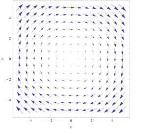
In vector calculus, the curl, also known as rotor, is a vector operator that describes the infinitesimal circulation of a vector field in three-dimensional Euclidean space. The curl at a point in the field is represented by a vector whose length and direction denote the magnitude and axis of the maximum circulation. The curl of a field is formally defined as the circulation density at each point of the field.
In vector calculus, divergence is a vector operator that operates on a vector field, producing a scalar field giving the quantity of the vector field's source at each point. More technically, the divergence represents the volume density of the outward flux of a vector field from an infinitesimal volume around a given point.
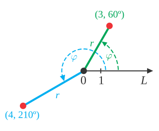
In mathematics, the polar coordinate system is a two-dimensional coordinate system in which each point on a plane is determined by a distance from a reference point and an angle from a reference direction. The reference point is called the pole, and the ray from the pole in the reference direction is the polar axis. The distance from the pole is called the radial coordinate, radial distance or simply radius, and the angle is called the angular coordinate, polar angle, or azimuth. Angles in polar notation are generally expressed in either degrees or radians.
In mathematics, a spherical coordinate system is a coordinate system for three-dimensional space where the position of a given point in space is specified by three numbers, : the radial distance of the radial liner connecting the point to the fixed point of origin ; the polar angle θ of the radial line r; and the azimuthal angle φ of the radial line r.
In mathematical analysis, the Dirac delta function, also known as the unit impulse, is a generalized function on the real numbers, whose value is zero everywhere except at zero, and whose integral over the entire real line is equal to one. Since there is no function having this property, to model the delta "function" rigorously involves the use of limits or, as is common in mathematics, measure theory and the theory of distributions.
The Navier–Stokes equations are partial differential equations which describe the motion of viscous fluid substances. They were named after French engineer and physicist Claude-Louis Navier and the Irish physicist and mathematician George Gabriel Stokes. They were developed over several decades of progressively building the theories, from 1822 (Navier) to 1842–1850 (Stokes).
In mathematics, Cauchy's integral formula, named after Augustin-Louis Cauchy, is a central statement in complex analysis. It expresses the fact that a holomorphic function defined on a disk is completely determined by its values on the boundary of the disk, and it provides integral formulas for all derivatives of a holomorphic function. Cauchy's formula shows that, in complex analysis, "differentiation is equivalent to integration": complex differentiation, like integration, behaves well under uniform limits – a result that does not hold in real analysis.
Noether's theorem states that every continuous symmetry of the action of a physical system with conservative forces has a corresponding conservation law. This is the first of two theorems proven by mathematician Emmy Noether in 1915 and published in 1918. The action of a physical system is the integral over time of a Lagrangian function, from which the system's behavior can be determined by the principle of least action. This theorem only applies to continuous and smooth symmetries of physical space.
In vector calculus, the Jacobian matrix of a vector-valued function of several variables is the matrix of all its first-order partial derivatives. When this matrix is square, that is, when the function takes the same number of variables as input as the number of vector components of its output, its determinant is referred to as the Jacobian determinant. Both the matrix and the determinant are often referred to simply as the Jacobian in literature.
In the mathematical field of differential geometry, a metric tensor is an additional structure on a manifold M that allows defining distances and angles, just as the inner product on a Euclidean space allows defining distances and angles there. More precisely, a metric tensor at a point p of M is a bilinear form defined on the tangent space at p, and a metric field on M consists of a metric tensor at each point p of M that varies smoothly with p.
In the calculus of variations, a field of mathematical analysis, the functional derivative relates a change in a functional to a change in a function on which the functional depends.
In mathematics, the Hodge star operator or Hodge star is a linear map defined on the exterior algebra of a finite-dimensional oriented vector space endowed with a nondegenerate symmetric bilinear form. Applying the operator to an element of the algebra produces the Hodge dual of the element. This map was introduced by W. V. D. Hodge.
The path integral formulation is a description in quantum mechanics that generalizes the stationary action principle of classical mechanics. It replaces the classical notion of a single, unique classical trajectory for a system with a sum, or functional integral, over an infinity of quantum-mechanically possible trajectories to compute a quantum amplitude.
In calculus, the Leibniz integral rule for differentiation under the integral sign states that for an integral of the form
In mathematics (specifically multivariable calculus), a multiple integral is a definite integral of a function of several real variables, for instance, f(x, y) or f(x, y, z). Physical (natural philosophy) interpretation: S any surface, V any volume, etc.. Incl. variable to time, position, etc.
The following are important identities involving derivatives and integrals in vector calculus.
In differential calculus, the Reynolds transport theorem, or simply the Reynolds theorem, named after Osborne Reynolds (1842–1912), is a three-dimensional generalization of the Leibniz integral rule. It is used to recast time derivatives of integrated quantities and is useful in formulating the basic equations of continuum mechanics.
In physics, Lagrangian mechanics is a formulation of classical mechanics founded on the stationary-action principle. It was introduced by the Italian-French mathematician and astronomer Joseph-Louis Lagrange in his presentation to the Turin Academy of Science in 1760 culminating in his 1788 grand opus, Mécanique analytique.
In classical mechanics, the central-force problem is to determine the motion of a particle in a single central potential field. A central force is a force that points from the particle directly towards a fixed point in space, the center, and whose magnitude only depends on the distance of the object to the center. In a few important cases, the problem can be solved analytically, i.e., in terms of well-studied functions such as trigonometric functions.
In mathematics, the Neumann–Poincaré operator or Poincaré–Neumann operator, named after Carl Neumann and Henri Poincaré, is a non-self-adjoint compact operator introduced by Poincaré to solve boundary value problems for the Laplacian on bounded domains in Euclidean space. Within the language of potential theory it reduces the partial differential equation to an integral equation on the boundary to which the theory of Fredholm operators can be applied. The theory is particularly simple in two dimensions—the case treated in detail in this article—where it is related to complex function theory, the conjugate Beurling transform or complex Hilbert transform and the Fredholm eigenvalues of bounded planar domains.
↑ Morris, Carla C. (2015-07-28). Fundamentals of calculus. Stark, Robert M., 1930-2017. Hoboken, New Jersey. ISBN9781119015314. OCLC893974565.{{cite book}}: CS1 maint: location missing publisher (link)
1 2 Weisstein, Eric W. "Differential Operator." From MathWorld--A Wolfram Web Resource. "Differential Operator". Archived from the original on 2016-01-21. Retrieved 2016-02-07.
↑ Weisstein, Eric W. "Repeated Integral." From MathWorld--A Wolfram Web Resource. "Repeated Integral". Archived from the original on 2016-02-01. Retrieved 2016-02-07.
1st to 7th, nth and (n+1)th derivatives: Method of Fluxions (Newton, 1736), pp. 313-318 and p. 265 (p. 163 in original MS: "Newton Papers: Fluxions". Archived from the original on 2017-04-06. Retrieved 2016-02-05.)
1st to 5th derivatives: A Treatise of Fluxions (Colin MacLaurin, 1742), p. 613
1st to 4th and nth derivatives: Articles "Differential" and "Fluxion", Dictionary of Pure and Mixed Mathematics (Peter Barlow, 1814)
1st to 6th and nth derivatives: The Mathematical Papers of Isaac Newton Vol. 7 1691-1695 (D. T. Whiteside, 1976), pp.88 and 17
1st to 3rd and nth derivatives: A History of Analysis (Hans Niels Jahnke, 2000), pp. 84-85
The dot for nth derivative may be omitted ( )
↑ Weisstein, Eric W. "Overdot." From MathWorld--A Wolfram Web Resource. "Overdot". Archived from the original on 2015-09-05. Retrieved 2016-02-05.
↑ Weisstein, Eric W. "Double Dot." From MathWorld--A Wolfram Web Resource. "Double Dot". Archived from the original on 2016-03-03. Retrieved 2016-02-05.
↑ Article 580 in Florian Cajori, A History of Mathematical Notations (1929), Dover Publications, Inc. New York. ISBN0-486-67766-4
↑ "Patterns of Mathematical Thought in the Later Seventeenth Century", Archive for History of Exact Sciences Vol. 1, No. 3 (D. T. Whiteside, 1961), pp. 361-362,378
↑ S.B. Engelsman has given more strict definitions in Families of Curves and the Origins of Partial Differentiation (2000), pp. 223-226
↑ Newton's notation for integration reproduced from:
1st to 3rd integrals: Method of Fluxions (Newton, 1736), pp. 265-266 (p. 163 in original MS: "Newton Papers: Fluxions". Archived from the original on 2017-04-06. Retrieved 2016-02-05.)
4th integrals: The Doctrine of Fluxions (James Hodgson, 1736), pp. 54 and 72
1st to 2nd integrals: Articles 622 and 365 in A History of Mathematical Notations (F .Cajori, 1929)
The nth integral notation is deducted from the nth derivative. It could be used in Methodus Incrementorum Directa & Inversa (Brook Taylor, 1715)
This page is based on this Wikipedia article Text is available under the CC BY-SA 4.0 license; additional terms may apply. Images, videos and audio are available under their respective licenses.