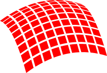
An illustration of a single surface element. These elements are made infinitesimally small, by the limiting process, so as to approximate the surface.
Surface integrals of scalar fields
Assume that f is a scalar, vector, or tensor field defined on a surface S. To find an explicit formula for the surface integral of f over S, we need to parameterizeS by defining a system of curvilinear coordinates on S, like the latitude and longitude on a sphere. Let such a parameterization be r(s, t), where (s, t) varies in some region T in the plane. Then, the surface integral is given by
where the expression between bars on the right-hand side is the magnitude of the cross product of the partial derivatives of r(s, t), and is known as the surface element (which would, for example, yield a smaller value near the poles of a sphere, where the lines of longitude converge more dramatically, and latitudinal coordinates are more compactly spaced). The surface integral can also be expressed in the equivalent form
For example, if we want to find the surface area of the graph of some scalar function, say z = f(x, y), we have
where r = (x, y, z) = (x, y, f(x, y)). So that , and . So,
which is the standard formula for the area of a surface described this way. One can recognize the vector in the second-last line above as the normal vector to the surface.
Because of the presence of the cross product, the above formulas only work for surfaces embedded in three-dimensional space.
A curved surface with a vector field passing through it. The red arrows (vectors) represent the magnitude and direction of the field at various points on the surface
Surface divided into small patches by a parameterization of the surface
The flux through each patch is equal to the normal (perpendicular) component of the field at the patch's location multiplied by the area . The normal component is equal to the dot product of with the unit normal vector (blue arrows)
The total flux through the surface is found by adding up for each patch. In the limit as the patches become infinitesimally small, this is the surface integral
Consider a vector field v on a surface S, that is, for each r = (x, y, z) in S, v(r) is a vector.
The integral of v on S was defined in the previous section. Suppose now that it is desired to integrate only the normal component of the vector field over the surface, the result being a scalar, usually called the flux passing through the surface. For example, imagine that we have a fluid flowing through S, such that v(r) determines the velocity of the fluid at r. The flux is defined as the quantity of fluid flowing through S per unit time.
This illustration implies that if the vector field is tangent to S at each point, then the flux is zero because the fluid just flows in parallel to S, and neither in nor out. This also implies that if v does not just flow along S, that is, if v has both a tangential and a normal component, then only the normal component contributes to the flux. Based on this reasoning, to find the flux, we need to take the dot product of v with the unit surface normaln to S at each point, which will give us a scalar field, and integrate the obtained field as above. In other words, we have to integrate v with respect to the vector surface element , which is the vector normal to S at the given point, whose magnitude is
We find the formula
The cross product on the right-hand side of this expression is a (not necessarily unital) surface normal determined by the parametrisation.
This formula defines the integral on the left (note the dot and the vector notation for the surface element).
We may also interpret this as a special case of integrating 2-forms, where we identify the vector field with a 1-form, and then integrate its Hodge dual over the surface. This is equivalent to integrating over the immersed surface, where is the induced volume form on the surface, obtained by interior multiplication of the Riemannian metric of the ambient space with the outward normal of the surface.
be an orientation preserving parametrization of S with in D. Changing coordinates from to , the differential forms transform as
So transforms to , where denotes the determinant of the Jacobian of the transition function from to . The transformation of the other forms are similar.
Then, the surface integral of f on S is given by
where
is the surface element normal to S.
Let us note that the surface integral of this 2-form is the same as the surface integral of the vector field which has as components , and .
Let us notice that we defined the surface integral by using a parametrization of the surface S. We know that a given surface might have several parametrizations. For example, if we move the locations of the North Pole and the South Pole on a sphere, the latitude and longitude change for all the points on the sphere. A natural question is then whether the definition of the surface integral depends on the chosen parametrization. For integrals of scalar fields, the answer to this question is simple; the value of the surface integral will be the same no matter what parametrization one uses.
For integrals of vector fields, things are more complicated because the surface normal is involved. It can be proven that given two parametrizations of the same surface, whose surface normals point in the same direction, one obtains the same value for the surface integral with both parametrizations. If, however, the normals for these parametrizations point in opposite directions, the value of the surface integral obtained using one parametrization is the negative of the one obtained via the other parametrization. It follows that given a surface, we do not need to stick to any unique parametrization, but, when integrating vector fields, we do need to decide in advance in which direction the normal will point and then choose any parametrization consistent with that direction.
Another issue is that sometimes surfaces do not have parametrizations which cover the whole surface. The obvious solution is then to split that surface into several pieces, calculate the surface integral on each piece, and then add them all up. This is indeed how things work, but when integrating vector fields, one needs to again be careful how to choose the normal-pointing vector for each piece of the surface, so that when the pieces are put back together, the results are consistent. For the cylinder, this means that if we decide that for the side region the normal will point out of the body, then for the top and bottom circular parts, the normal must point out of the body too.
Last, there are surfaces which do not admit a surface normal at each point with consistent results (for example, the Möbius strip). If such a surface is split into pieces, on each piece a parametrization and corresponding surface normal is chosen, and the pieces are put back together, we will find that the normal vectors coming from different pieces cannot be reconciled. This means that at some junction between two pieces we will have normal vectors pointing in opposite directions. Such a surface is called non-orientable, and on this kind of surface, one cannot talk about integrating vector fields.
In vector calculus, the curl, also known as rotor, is a vector operator that describes the infinitesimal circulation of a vector field in three-dimensional Euclidean space. The curl at a point in the field is represented by a vector whose length and direction denote the magnitude and axis of the maximum circulation. The curl of a field is formally defined as the circulation density at each point of the field.
In vector calculus and differential geometry the generalized Stokes theorem, also called the Stokes–Cartan theorem, is a statement about the integration of differential forms on manifolds, which both simplifies and generalizes several theorems from vector calculus. In particular, the fundamental theorem of calculus is the special case where the manifold is a line segment, Green’s theorem and Stokes' theorem are the cases of a surface in or and the divergence theorem is the case of a volume in Hence, the theorem is sometimes referred to as the Fundamental Theorem of Multivariate Calculus.
Flux describes any effect that appears to pass or travel through a surface or substance. Flux is a concept in applied mathematics and vector calculus which has many applications to physics. For transport phenomena, flux is a vector quantity, describing the magnitude and direction of the flow of a substance or property. In vector calculus flux is a scalar quantity, defined as the surface integral of the perpendicular component of a vector field over a surface.
In mathematics, curvature is any of several strongly related concepts in geometry. Intuitively, the curvature is the amount by which a curve deviates from being a straight line, or a surface deviates from being a plane.
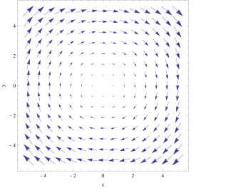
In vector calculus and physics, a vector field is an assignment of a vector to each point in a space, most commonly Euclidean space . A vector field on a plane can be visualized as a collection of arrows with given magnitudes and directions, each attached to a point on the plane. Vector fields are often used to model, for example, the speed and direction of a moving fluid throughout three dimensional space, such as the wind, or the strength and direction of some force, such as the magnetic or gravitational force, as it changes from one point to another point.
In mathematics, Cauchy's integral formula, named after Augustin-Louis Cauchy, is a central statement in complex analysis. It expresses the fact that a holomorphic function defined on a disk is completely determined by its values on the boundary of the disk, and it provides integral formulas for all derivatives of a holomorphic function. Cauchy's formula shows that, in complex analysis, "differentiation is equivalent to integration": complex differentiation, like integration, behaves well under uniform limits – a result that does not hold in real analysis.
In vector calculus, the divergence theorem, also known as Gauss's theorem or Ostrogradsky's theorem, is a theorem which relates the flux of a vector field through a closed surface to the divergence of the field in the volume enclosed.
In geometry, a normal is an object that is perpendicular to a given object. For example, the normal line to a plane curve at a given point is the line perpendicular to the tangent line to the curve at the point.
In vector calculus, Green's theorem relates a line integral around a simple closed curve C to a double integral over the plane region D bounded by C. It is the two-dimensional special case of Stokes' theorem.
In mathematical physics, scalar potential, simply stated, describes the situation where the difference in the potential energies of an object in two different positions depends only on the positions, not upon the path taken by the object in traveling from one position to the other. It is a scalar field in three-space: a directionless value (scalar) that depends only on its location. A familiar example is potential energy due to gravity.
In classical electromagnetism, magnetic vector potential is the vector quantity defined so that its curl is equal to the magnetic field: . Together with the electric potential φ, the magnetic vector potential can be used to specify the electric field E as well. Therefore, many equations of electromagnetism can be written either in terms of the fields E and B, or equivalently in terms of the potentials φ and A. In more advanced theories such as quantum mechanics, most equations use potentials rather than fields.
In geometry, a three-dimensional space is a mathematical space in which three values (coordinates) are required to determine the position of a point. Most commonly, it is the three-dimensional Euclidean space, that is, the Euclidean space of dimension three, which models physical space. More general three-dimensional spaces are called 3-manifolds. The term may also refer colloquially to a subset of space, a three-dimensional region, a solid figure.
The following are important identities involving derivatives and integrals in vector calculus.
A parametric surface is a surface in the Euclidean space which is defined by a parametric equation with two parameters :\mathbb {R} ^{2}\to \mathbb {R} ^{3}} . Parametric representation is a very general way to specify a surface, as well as implicit representation. Surfaces that occur in two of the main theorems of vector calculus, Stokes' theorem and the divergence theorem, are frequently given in a parametric form. The curvature and arc length of curves on the surface, surface area, differential geometric invariants such as the first and second fundamental forms, Gaussian, mean, and principal curvatures can all be computed from a given parametrization.
A vector-valued function, also referred to as a vector function, is a mathematical function of one or more variables whose range is a set of multidimensional vectors or infinite-dimensional vectors. The input of a vector-valued function could be a scalar or a vector ; the dimension of the function's domain has no relation to the dimension of its range.
The gradient theorem, also known as the fundamental theorem of calculus for line integrals, says that a line integral through a gradient field can be evaluated by evaluating the original scalar field at the endpoints of the curve. The theorem is a generalization of the second fundamental theorem of calculus to any curve in a plane or space rather than just the real line.
In differential calculus, there is no single uniform notation for differentiation. Instead, various notations for the derivative of a function or variable have been proposed by various mathematicians. The usefulness of each notation varies with the context, and it is sometimes advantageous to use more than one notation in a given context. The most common notations for differentiation are listed below.
In mathematics, a line integral is an integral where the function to be integrated is evaluated along a curve. The terms path integral, curve integral, and curvilinear integral are also used; contour integral is used as well, although that is typically reserved for line integrals in the complex plane.
Stokes' theorem, also known as the Kelvin–Stokes theorem after Lord Kelvin and George Stokes, the fundamental theorem for curls or simply the curl theorem, is a theorem in vector calculus on . Given a vector field, the theorem relates the integral of the curl of the vector field over some surface, to the line integral of the vector field around the boundary of the surface. The classical theorem of Stokes can be stated in one sentence: The line integral of a vector field over a loop is equal to its curl through the enclosed surface. It is illustrated in the figure, where the direction of positive circulation of the bounding contour ∂Σ, and the direction n of positive flux through the surface Σ, are related by a right-hand-rule. For the right hand the fingers circulate along ∂Σ and the thumb is directed along n.
Lagrangian field theory is a formalism in classical field theory. It is the field-theoretic analogue of Lagrangian mechanics. Lagrangian mechanics is used to analyze the motion of a system of discrete particles each with a finite number of degrees of freedom. Lagrangian field theory applies to continua and fields, which have an infinite number of degrees of freedom.
References
↑ Edwards, C. H. (1994). Advanced Calculus of Several Variables. Mineola, NY: Dover. p.335. ISBN0-486-68336-2.
This page is based on this Wikipedia article Text is available under the CC BY-SA 4.0 license; additional terms may apply. Images, videos and audio are available under their respective licenses.