A continuous function on the closed interval showing the absolute max (red) and the absolute min (blue).
In calculus, the extreme value theorem states that if a real-valued function is continuous on the closed and bounded interval , then must attain a maximum and a minimum, each at least once. That is, there exist numbers and in such that:
The extreme value theorem is more specific than the related boundedness theorem, which states merely that a continuous function on the closed interval is bounded on that interval; that is, there exist real numbers and such that:
This does not say that and are necessarily the maximum and minimum values of on the interval which is what the extreme value theorem stipulates must also be the case.
The extreme value theorem was originally proven by Bernard Bolzano in the 1830s in a work Function Theory but the work remained unpublished until 1930. Bolzano's proof consisted of showing that a continuous function on a closed interval was bounded, and then showing that the function attained a maximum and a minimum value. Both proofs involved what is known today as the Bolzano–Weierstrass theorem.[1]
Functions to which the theorem does not apply
The following examples show why the function domain must be closed and bounded in order for the theorem to apply. Each fails to attain a maximum on the given interval.
defined over is not bounded from above.
defined over is bounded but does not attain its least upper bound .
defined over is not bounded from above.
defined over is bounded but never attains its least upper bound .
Defining in the last two examples shows that both theorems require continuity on .
Generalization to metric and topological spaces
When moving from the real line to metric spaces and general topological spaces, the appropriate generalization of a closed bounded interval is a compact set. A set is said to be compact if it has the following property: from every collection of open sets such that , a finite subcollection can be chosen such that . This is usually stated in short as "every open cover of has a finite subcover". The Heine–Borel theorem asserts that a subset of the real line is compact if and only if it is both closed and bounded. Correspondingly, a metric space has the Heine–Borel property if every closed and bounded set is also compact.
The concept of a continuous function can likewise be generalized. Given topological spaces , a function is said to be continuous if for every open set , is also open. Given these definitions, continuous functions can be shown to preserve compactness:[2]
Theorem.If are topological spaces, is a continuous function, and is compact, then is also compact.
In particular, if , then this theorem implies that is closed and bounded for any compact set , which in turn implies that attains its supremum and infimum on any (nonempty) compact set . Thus, we have the following generalization of the extreme value theorem:[2]
Theorem.Ifis a compact set andis a continuous function, thenis bounded and there existsuch thatand.
We look at the proof for the upper bound and the maximum of . By applying these results to the function , the existence of the lower bound and the result for the minimum of follows. Also note that everything in the proof is done within the context of the real numbers.
We first prove the boundedness theorem, which is a step in the proof of the extreme value theorem. The basic steps involved in the proof of the extreme value theorem are:
Prove the boundedness theorem.
Find a sequence so that its image converges to the supremum of .
Show that there exists a subsequence that converges to a point in the domain.
Use continuity to show that the image of the subsequence converges to the supremum.
Proof of the boundedness theorem
StatementIf is continuous on then it is bounded on
Suppose the function is not bounded above on the interval . Then, for every natural number , there exists an such that . This defines a sequence. Because is bounded, the Bolzano–Weierstrass theorem implies that there exists a convergent subsequence of . Denote its limit by . As is closed, it contains . Because is continuous at , we know that converges to the real number (as is sequentially continuous at ). But for every , which implies that diverges to , a contradiction. Therefore, is bounded above on .
Alternative proof
StatementIf is continuous on then it is bounded on
Proof Consider the set of points in such that is bounded on . We note that is one such point, for is bounded on by the value . If is another point, then all points between and also belong to . In other words is an interval closed at its left end by .
Now is continuous on the right at , hence there exists such that for all in . Thus is bounded by and on the interval so that all these points belong to .
So far, we know that is an interval of non-zero length, closed at its left end by .
Next, is bounded above by . Hence the set has a supremum in ; let us call it . From the non-zero length of we can deduce that .
Suppose . Now is continuous at , hence there exists such that for all in so that is bounded on this interval. But it follows from the supremacy of that there exists a point belonging to , say, which is greater than . Thus is bounded on which overlaps so that is bounded on . This however contradicts the supremacy of .
We must therefore have . Now is continuous on the left at , hence there exists such that for all in so that is bounded on this interval. But it follows from the supremacy of that there exists a point belonging to , say, which is greater than . Thus is bounded on which overlaps so that is bounded on .∎
Proof of the extreme value theorem
By the boundedness theorem, f is bounded from above, hence, by the Dedekind-completeness of the real numbers, the least upper bound (supremum) M of f exists. It is necessary to find a point d in [a, b] such that M = f(d). Let n be a natural number. As M is the least upper bound, M – 1/n is not an upper bound for f. Therefore, there exists dn in [a, b] so that M – 1/n < f(dn). This defines a sequence {dn}. Since M is an upper bound for f, we have M – 1/n < f(dn) ≤ M for all n. Therefore, the sequence {f(dn)} converges to M.
The Bolzano–Weierstrass theorem tells us that there exists a subsequence {}, which converges to some d and, as [a, b] is closed, d is in [a, b]. Since f is continuous at d, the sequence {f()} converges to f(d). But {f(dnk)} is a subsequence of {f(dn)} that converges to M, so M = f(d). Therefore, f attains its supremum M at d.∎
Alternative proof of the extreme value theorem
The set {y∈R: y = f(x) for some x∈ [a,b]} is a bounded set. Hence, its least upper bound exists by least upper bound property of the real numbers. Let M = sup(f(x))on[a, b]. If there is no point x on [a,b] so that f(x)=M, then f(x) < M on [a,b]. Therefore, 1/(M−f(x)) is continuous on [a, b].
However, to every positive number ε, there is always some x in [a,b] such that M−f(x) < ε because M is the least upper bound. Hence, 1/(M−f(x)) > 1/ε, which means that 1/(M−f(x)) is not bounded. Since every continuous function on a [a, b] is bounded, this contradicts the conclusion that 1/(M−f(x)) was continuous on [a,b]. Therefore, there must be a point x in [a,b] such that f(x)=M. ∎
Proof using the hyperreals
In the setting of non-standard calculus, let N be an infinite hyperinteger. The interval [0,1] has a natural hyperreal extension. Consider its partition into N subintervals of equal infinitesimal length 1/N, with partition points xi= i/N as i "runs" from 0 to N. The function ƒ is also naturally extended to a function ƒ* defined on the hyperreals between 0 and 1. Note that in the standard setting (when N is finite), a point with the maximal value of ƒ can always be chosen among the N+1 points xi, by induction. Hence, by the transfer principle, there is a hyperinteger i0 such that 0≤ i0≤ N and for all i=0,...,N. Consider the real point
where st is the standard part function. An arbitrary real point x lies in a suitable sub-interval of the partition, namely , so thatst(xi)= x. Applying st to the inequality , we obtain . By continuity of ƒ we have
.
Hence ƒ(c)≥ ƒ(x), for all real x, proving c to be a maximum of ƒ.[3]
Proof from first principles
Statement If is continuous on then it attains its supremum on
Proof By the Boundedness Theorem, is bounded above on and by the completeness property of the real numbers has a supremum in . Let us call it , or . It is clear that the restriction of to the subinterval where has a supremum which is less than or equal to , and that increases from to as increases from to .
If then we are done. Suppose therefore that and let . Consider the set of points in such that .
Clearly ; moreover if is another point in then all points between and also belong to because is monotonic increasing. Hence is a non-empty interval, closed at its left end by .
Now is continuous on the right at , hence there exists such that for all in . Thus is less than on the interval so that all these points belong to .
Next, is bounded above by and has therefore a supremum in : let us call it . We see from the above that . We will show that is the point we are seeking i.e. the point where attains its supremum, or in other words .
Suppose the contrary viz. . Let and consider the following two cases:
. As is continuous at , there exists such that for all in . This means that is less than on the interval . But it follows from the supremacy of that there exists a point, say, belonging to which is greater than . By the definition of , . Let then for all in , . Taking to be the minimum of and , we have for all in . Hence so that . This however contradicts the supremacy of and completes the proof.
. As is continuous on the left at , there exists such that for all in . This means that is less than on the interval . But it follows from the supremacy of that there exists a point, say, belonging to which is greater than . By the definition of , . Let then for all in , . Taking to be the minimum of and , we have for all in . This contradicts the supremacy of and completes the proof.
Extension to semi-continuous functions
If the continuity of the function f is weakened to semi-continuity, then the corresponding half of the boundedness theorem and the extreme value theorem hold and the values –∞ or +∞, respectively, from the extended real number line can be allowed as possible values. More precisely:
Theorem: If a function f: [a, b] → [–∞, ∞) is upper semi-continuous, meaning that
for all x in [a,b], then f is bounded above and attains its supremum.
Proof: If f(x) = –∞ for all x in [a,b], then the supremum is also –∞ and the theorem is true. In all other cases, the proof is a slight modification of the proofs given above. In the proof of the boundedness theorem, the upper semi-continuity of f at x only implies that the limit superior of the subsequence {f(xnk)} is bounded above by f(x) < ∞, but that is enough to obtain the contradiction. In the proof of the extreme value theorem, upper semi-continuity of f at d implies that the limit superior of the subsequence {f(dnk)} is bounded above by f(d), but this suffices to conclude that f(d) = M.∎
Applying this result to −f proves:
Theorem: If a function f: [a, b] → (–∞, ∞] is lower semi-continuous, meaning that
for all x in [a,b], then f is bounded below and attains its infimum.
A real-valued function is upper as well as lower semi-continuous, if and only if it is continuous in the usual sense. Hence these two theorems imply the boundedness theorem and the extreme value theorem.
Related Research Articles
Brouwer's fixed-point theorem is a fixed-point theorem in topology, named after L. E. J. (Bertus) Brouwer. It states that for any continuous function mapping a nonempty compact convex set to itself, there is a point such that . The simplest forms of Brouwer's theorem are for continuous functions from a closed interval in the real numbers to itself or from a closed disk to itself. A more general form than the latter is for continuous functions from a nonempty convex compact subset of Euclidean space to itself.
In mathematics, especially functional analysis, a Banach algebra, named after Stefan Banach, is an associative algebra over the real or complex numbers that at the same time is also a Banach space, that is, a normed space that is complete in the metric induced by the norm. The norm is required to satisfy
In mathematics, specifically general topology, compactness is a property that seeks to generalize the notion of a closed and bounded subset of Euclidean space. The idea is that a compact space has no "punctures" or "missing endpoints", i.e., it includes all limiting values of points. For example, the open interval (0,1) would not be compact because it excludes the limiting values of 0 and 1, whereas the closed interval [0,1] would be compact. Similarly, the space of rational numbers is not compact, because it has infinitely many "punctures" corresponding to the irrational numbers, and the space of real numbers is not compact either, because it excludes the two limiting values and . However, the extended real number linewould be compact, since it contains both infinities. There are many ways to make this heuristic notion precise. These ways usually agree in a metric space, but may not be equivalent in other topological spaces.
In mathematics, a continuous function is a function such that a small variation of the argument induces a small variation of the value of the function. This implies there are no abrupt changes in value, known as discontinuities. More precisely, a function is continuous if arbitrarily small changes in its value can be assured by restricting to sufficiently small changes of its argument. A discontinuous function is a function that is not continuous. Until the 19th century, mathematicians largely relied on intuitive notions of continuity and considered only continuous functions. The epsilon–delta definition of a limit was introduced to formalize the definition of continuity.
In mathematical analysis, the intermediate value theorem states that if is a continuous function whose domain contains the interval [a, b], then it takes on any given value between and at some point within the interval.
In the branch of mathematics known as real analysis, the Riemann integral, created by Bernhard Riemann, was the first rigorous definition of the integral of a function on an interval. It was presented to the faculty at the University of Göttingen in 1854, but not published in a journal until 1868. For many functions and practical applications, the Riemann integral can be evaluated by the fundamental theorem of calculus or approximated by numerical integration, or simulated using Monte Carlo integration.
In mathematics, the branch of real analysis studies the behavior of real numbers, sequences and series of real numbers, and real functions. Some particular properties of real-valued sequences and functions that real analysis studies include convergence, limits, continuity, smoothness, differentiability and integrability.
In mathematical analysis, the Weierstrass approximation theorem states that every continuous function defined on a closed interval [a, b] can be uniformly approximated as closely as desired by a polynomial function. Because polynomials are among the simplest functions, and because computers can directly evaluate polynomials, this theorem has both practical and theoretical relevance, especially in polynomial interpolation. The original version of this result was established by Karl Weierstrass in 1885 using the Weierstrass transform.
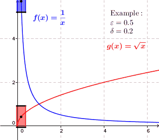
In mathematics, a real function of real numbers is said to be uniformly continuous if there is a positive real number such that function values over any function domain interval of the size are as close to each other as we want. In other words, for a uniformly continuous real function of real numbers, if we want function value differences to be less than any positive real number , then there is a positive real number such that at any and in any function interval of the size .
In the mathematical field of analysis, uniform convergence is a mode of convergence of functions stronger than pointwise convergence, in the sense that the convergence is uniform over the domain. A sequence of functions converges uniformly to a limiting function on a set as the function domain if, given any arbitrarily small positive number , a number can be found such that each of the functions differs from by no more than at every pointin. Described in an informal way, if converges to uniformly, then how quickly the functions approach is "uniform" throughout in the following sense: in order to guarantee that differs from by less than a chosen distance , we only need to make sure that is larger than or equal to a certain , which we can find without knowing the value of in advance. In other words, there exists a number that could depend on but is independent of , such that choosing will ensure that for all . In contrast, pointwise convergence of to merely guarantees that for any given in advance, we can find such that, for that particular, falls within of whenever .
In mathematics, mathematical physics and the theory of stochastic processes, a harmonic function is a twice continuously differentiable function where U is an open subset of that satisfies Laplace's equation, that is,
In vector calculus, Green's theorem relates a line integral around a simple closed curve C to a double integral over the plane region D bounded by C. It is the two-dimensional special case of Stokes' theorem.
In mathematics, the uniform boundedness principle or Banach–Steinhaus theorem is one of the fundamental results in functional analysis. Together with the Hahn–Banach theorem and the open mapping theorem, it is considered one of the cornerstones of the field. In its basic form, it asserts that for a family of continuous linear operators whose domain is a Banach space, pointwise boundedness is equivalent to uniform boundedness in operator norm.
In calculus and real analysis, absolute continuity is a smoothness property of functions that is stronger than continuity and uniform continuity. The notion of absolute continuity allows one to obtain generalizations of the relationship between the two central operations of calculus—differentiation and integration. This relationship is commonly characterized in the framework of Riemann integration, but with absolute continuity it may be formulated in terms of Lebesgue integration. For real-valued functions on the real line, two interrelated notions appear: absolute continuity of functions and absolute continuity of measures. These two notions are generalized in different directions. The usual derivative of a function is related to the Radon–Nikodym derivative, or density, of a measure. We have the following chains of inclusions for functions over a compact subset of the real line:
In mathematics, a function f defined on some set X with real or complex values is called bounded if the set of its values is bounded. In other words, there exists a real number M such that
In mathematical analysis, a family of functions is equicontinuous if all the functions are continuous and they have equal variation over a given neighbourhood, in a precise sense described herein. In particular, the concept applies to countable families, and thus sequences of functions.
The Arzelà–Ascoli theorem is a fundamental result of mathematical analysis giving necessary and sufficient conditions to decide whether every sequence of a given family of real-valued continuous functions defined on a closed and bounded interval has a uniformly convergent subsequence. The main condition is the equicontinuity of the family of functions. The theorem is the basis of many proofs in mathematics, including that of the Peano existence theorem in the theory of ordinary differential equations, Montel's theorem in complex analysis, and the Peter–Weyl theorem in harmonic analysis and various results concerning compactness of integral operators.
In mathematics, nonstandard calculus is the modern application of infinitesimals, in the sense of nonstandard analysis, to infinitesimal calculus. It provides a rigorous justification for some arguments in calculus that were previously considered merely heuristic.
In mathematics, a function is locally bounded if it is bounded around every point. A family of functions is locally bounded if for any point in their domain all the functions are bounded around that point and by the same number.
The fundamental theorem of calculus is a theorem that links the concept of differentiating a function with the concept of integrating a function. The two operations are inverses of each other apart from a constant value which depends on where one starts to compute area.
References
↑ Rusnock, Paul; Kerr-Lawson, Angus (2005). "Bolzano and Uniform Continuity". Historia Mathematica. 32 (3): 303–311. doi:10.1016/j.hm.2004.11.003.
This page is based on this Wikipedia article Text is available under the CC BY-SA 4.0 license; additional terms may apply. Images, videos and audio are available under their respective licenses.
![A continuous function
f
(
x
)
{\displaystyle f(x)}
on the closed interval
[
a
,
b
]
{\displaystyle [a,b]}
showing the absolute max (red) and the absolute min (blue). Extreme Value Theorem.svg](http://upload.wikimedia.org/wikipedia/commons/thumb/0/00/Extreme_Value_Theorem.svg/300px-Extreme_Value_Theorem.svg.png)