
In vector calculus, divergence is a vector operator that operates on a vector field, producing a scalar field giving the quantity of the vector field's source at each point. More technically, the divergence represents the volume density of the outward flux of a vector field from an infinitesimal volume around a given point.
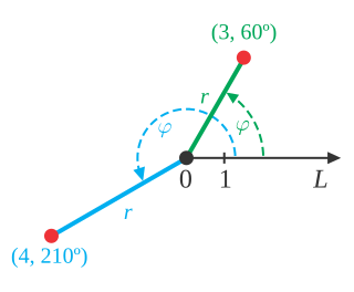
In mathematics, the polar coordinate system is a two-dimensional coordinate system in which each point on a plane is determined by a distance from a reference point and an angle from a reference direction. The reference point is called the pole, and the ray from the pole in the reference direction is the polar axis. The distance from the pole is called the radial coordinate, radial distance or simply radius, and the angle is called the angular coordinate, polar angle, or azimuth. Angles in polar notation are generally expressed in either degrees or radians.

In mathematics, a spherical coordinate system is a coordinate system for three-dimensional space where the position of a given point in space is specified by three numbers, : the radial distance of the radial liner connecting the point to the fixed point of origin ; the polar angle θ of the radial line r; and the azimuthal angle φ of the radial line r.

In mathematics and physics, Laplace's equation is a second-order partial differential equation named after Pierre-Simon Laplace, who first studied its properties. This is often written as

The Navier–Stokes equations are partial differential equations which describe the motion of viscous fluid substances. They were named after French engineer and physicist Claude-Louis Navier and the Irish physicist and mathematician George Gabriel Stokes. They were developed over several decades of progressively building the theories, from 1822 (Navier) to 1842–1850 (Stokes).
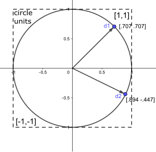
In mathematics, a unit vector in a normed vector space is a vector of length 1. A unit vector is often denoted by a lowercase letter with a circumflex, or "hat", as in .
In mathematics, the Laplace operator or Laplacian is a differential operator given by the divergence of the gradient of a scalar function on Euclidean space. It is usually denoted by the symbols , (where is the nabla operator), or . In a Cartesian coordinate system, the Laplacian is given by the sum of second partial derivatives of the function with respect to each independent variable. In other coordinate systems, such as cylindrical and spherical coordinates, the Laplacian also has a useful form. Informally, the Laplacian Δf (p) of a function f at a point p measures by how much the average value of f over small spheres or balls centered at p deviates from f (p).
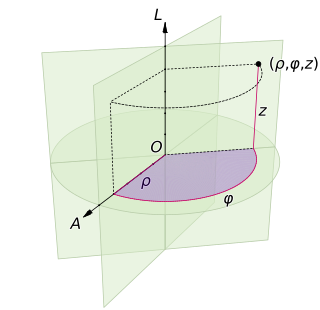
A cylindrical coordinate system is a three-dimensional coordinate system that specifies point positions by the distance from a chosen reference axis (axis L in the image opposite), the direction from the axis relative to a chosen reference direction (axis A), and the distance from a chosen reference plane perpendicular to the axis (plane containing the purple section). The latter distance is given as a positive or negative number depending on which side of the reference plane faces the point.
In vector calculus, the Jacobian matrix of a vector-valued function of several variables is the matrix of all its first-order partial derivatives. When this matrix is square, that is, when the function takes the same number of variables as input as the number of vector components of its output, its determinant is referred to as the Jacobian determinant. Both the matrix and the determinant are often referred to simply as the Jacobian in literature.
In the mathematical field of differential geometry, a metric tensor is an additional structure on a manifold M that allows defining distances and angles, just as the inner product on a Euclidean space allows defining distances and angles there. More precisely, a metric tensor at a point p of M is a bilinear form defined on the tangent space at p, and a metric field on M consists of a metric tensor at each point p of M that varies smoothly with p.
In the calculus of variations, a field of mathematical analysis, the functional derivative relates a change in a functional to a change in a function on which the functional depends.
This is a list of some vector calculus formulae for working with common curvilinear coordinate systems.
In general relativity, the metric tensor is the fundamental object of study. The metric captures all the geometric and causal structure of spacetime, being used to define notions such as time, distance, volume, curvature, angle, and separation of the future and the past.

In mathematics (specifically multivariable calculus), a multiple integral is a definite integral of a function of several real variables, for instance, f(x, y) or f(x, y, z). Physical (natural philosophy) interpretation: S any surface, V any volume, etc.. Incl. variable to time, position, etc.
The Mason–Weaver equation describes the sedimentation and diffusion of solutes under a uniform force, usually a gravitational field. Assuming that the gravitational field is aligned in the z direction, the Mason–Weaver equation may be written

There are various mathematical descriptions of the electromagnetic field that are used in the study of electromagnetism, one of the four fundamental interactions of nature. In this article, several approaches are discussed, although the equations are in terms of electric and magnetic fields, potentials, and charges with currents, generally speaking.
In applied mathematics, discontinuous Galerkin methods (DG methods) form a class of numerical methods for solving differential equations. They combine features of the finite element and the finite volume framework and have been successfully applied to hyperbolic, elliptic, parabolic and mixed form problems arising from a wide range of applications. DG methods have in particular received considerable interest for problems with a dominant first-order part, e.g. in electrodynamics, fluid mechanics and plasma physics. Indeed, the solutions of such problems may involve strong gradients (and even discontinuities) so that classical finite element methods fail, while finite volume methods are restricted to low order approximations.
In mathematics, the spectral theory of ordinary differential equations is the part of spectral theory concerned with the determination of the spectrum and eigenfunction expansion associated with a linear ordinary differential equation. In his dissertation, Hermann Weyl generalized the classical Sturm–Liouville theory on a finite closed interval to second order differential operators with singularities at the endpoints of the interval, possibly semi-infinite or infinite. Unlike the classical case, the spectrum may no longer consist of just a countable set of eigenvalues, but may also contain a continuous part. In this case the eigenfunction expansion involves an integral over the continuous part with respect to a spectral measure, given by the Titchmarsh–Kodaira formula. The theory was put in its final simplified form for singular differential equations of even degree by Kodaira and others, using von Neumann's spectral theorem. It has had important applications in quantum mechanics, operator theory and harmonic analysis on semisimple Lie groups.
Lagrangian field theory is a formalism in classical field theory. It is the field-theoretic analogue of Lagrangian mechanics. Lagrangian mechanics is used to analyze the motion of a system of discrete particles each with a finite number of degrees of freedom. Lagrangian field theory applies to continua and fields, which have an infinite number of degrees of freedom.


