Riemann sum

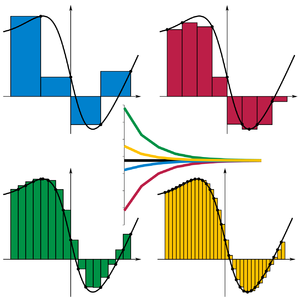
Four of the methods for approximating the area under curves. Left and right methods make the approximation using the right and left endpoints of each subinterval, respectively. Upper and lower methods make the approximation using the largest and smallest endpoint values of each subinterval, respectively. The values of the sums converge as the subintervals halve from top-left to bottom-right.

In mathematics, a Riemann sum is a certain kind of approximation of an integral by a finite sum. It is named after nineteenth century German mathematician Bernhard Riemann. One very common application is in numerical integration, i.e., approximating the area of functions or lines on a graph, where it is also known as the rectangle rule. It can also be applied for approximating the length of curves and other approximations.

The sum is calculated by partitioning the region into shapes (rectangles, trapezoids, parabolas, or cubics — sometimes infinitesimally small) that together form a region that is similar to the region being measured, then calculating the area for each of these shapes, and finally adding all of these small areas together. This approach can be used to find a numerical approximation for a definite integral even if the fundamental theorem of calculus does not make it easy to find a closed-form solution.

Because the region by the small shapes is usually not exactly the same shape as the region being measured, the Riemann sum will differ from the area being measured. This error can be reduced by dividing up the region more finely, using smaller and smaller shapes. As the shapes get smaller and smaller, the sum approaches the Riemann integral.

Definition

Let ${\displaystyle f:[a,b]\to \mathbb {R} }$ be a function defined on a closed interval ${\displaystyle [a,b]}$ of the real numbers, ${\displaystyle \mathbb {R} }$, and ${\displaystyle P=(x_{0},x_{1},\ldots ,x_{n})}$ as a partition of ${\displaystyle [a,b]}$, that is

$${\displaystyle a=x_{0}<x_{1}<x_{2}<\dots <x_{n}=b.}$$

A Riemann sum${\displaystyle S}$ of ${\displaystyle f}$ over ${\displaystyle [a,b]}$ with partition ${\displaystyle P}$ is defined as

$${\displaystyle S=\sum _{i=1}^{n}f(x_{i}^{*})\,\Delta x_{i},}$$

where ${\displaystyle \Delta x_{i}=x_{i}-x_{i-1}}$ and ${\displaystyle x_{i}^{*}\in [x_{i-1},x_{i}]}$. ^[1] One might produce different Riemann sums depending on which ${\displaystyle x_{i}^{*}}$'s are chosen. In the end this will not matter, if the function is Riemann integrable, when the difference or width of the summands ${\displaystyle \Delta x_{i}}$ approaches zero.

Types of Riemann sums

Specific choices of ${\displaystyle x_{i}^{*}}$ give different types of Riemann sums:

• If ${\displaystyle x_{i}^{*}=x_{i-1}}$ for all i, the method is the left rule ^{[2] [3]} and gives a left Riemann sum.
• If ${\displaystyle x_{i}^{*}=x_{i}}$ for all i, the method is the right rule ^{[2] [3]} and gives a right Riemann sum.
• If ${\displaystyle x_{i}^{*}=(x_{i}+x_{i-1})/2}$ for all i, the method is the midpoint rule ^{[2] [3]} and gives a middle Riemann sum.
• If ${\displaystyle f(x_{i}^{*})=\sup f([x_{i-1},x_{i}])}$ (that is, the supremum of${\textstyle f}$ over ${\displaystyle [x_{i-1},x_{i}]}$), the method is the upper rule and gives an upper Riemann sum or upper Darboux sum.
• If ${\displaystyle f(x_{i}^{*})=\inf f([x_{i-1},x_{i}])}$ (that is, the infimum of f over ${\displaystyle [x_{i-1},x_{i}]}$), the method is the lower rule and gives a lower Riemann sum or lower Darboux sum.

All these Riemann summation methods are among the most basic ways to accomplish numerical integration. Loosely speaking, a function is Riemann integrable if all Riemann sums converge as the partition "gets finer and finer".

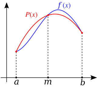
While not derived as a Riemann sum, taking the average of the left and right Riemann sums is the trapezoidal rule and gives a trapezoidal sum. It is one of the simplest of a very general way of approximating integrals using weighted averages. This is followed in complexity by Simpson's rule and Newton–Cotes formulas.

Any Riemann sum on a given partition (that is, for any choice of ${\displaystyle x_{i}^{*}}$ between ${\displaystyle x_{i-1}}$ and ${\displaystyle x_{i}}$) is contained between the lower and upper Darboux sums. This forms the basis of the Darboux integral, which is ultimately equivalent to the Riemann integral.

Riemann summation methods

The four Riemann summation methods are usually best approached with subintervals of equal size. The interval [a, b] is therefore divided into ${\displaystyle n}$ subintervals, each of length

$${\displaystyle \Delta x={\frac {b-a}{n}}.}$$

The points in the partition will then be

$${\displaystyle a,\;a+\Delta x,\;a+2\Delta x,\;\ldots ,\;a+(n-2)\Delta x,\;a+(n-1)\Delta x,\;b.}$$

Left rule

Left Riemann sum of x ↦ x over [0, 2] using 4 subintervals

For the left rule, the function is approximated by its values at the left endpoints of the subintervals. This gives multiple rectangles with base Δx and height f(a + iΔx). Doing this for i = 0, 1, ..., n − 1, and summing the resulting areas gives

$${\displaystyle S_{\mathrm {left} }=\Delta x\left[f(a)+f(a+\Delta x)+f(a+2\Delta x)+\dots +f(b-\Delta x)\right].}$$

The left Riemann sum amounts to an overestimation if f is monotonically decreasing on this interval, and an underestimation if it is monotonically increasing. The error of this formula will be

$${\displaystyle \left\vert \int _{a}^{b}f(x)\,dx-S_{\mathrm {left} }\right\vert \leq {\frac {M_{1}(b-a)^{2}}{2n}},}$$

where ${\displaystyle M_{1}}$ is the maximum value of the absolute value of ${\displaystyle f^{\prime }(x)}$ over the interval.

Right rule

Right Riemann sum of x ↦ x over [0, 2] using 4 subintervals

For the right rule, the function is approximated by its values at the right endpoints of the subintervals. This gives multiple rectangles with base Δx and height f(a + iΔx). Doing this for i = 1, ..., n, and summing the resulting areas gives

$${\displaystyle S_{\mathrm {right} }=\Delta x\left[f(a+\Delta x)+f(a+2\Delta x)+\dots +f(b)\right].}$$

The right Riemann sum amounts to an underestimation if f is monotonically decreasing, and an overestimation if it is monotonically increasing. The error of this formula will be

$${\displaystyle \left\vert \int _{a}^{b}f(x)\,dx-S_{\mathrm {right} }\right\vert \leq {\frac {M_{1}(b-a)^{2}}{2n}},}$$

where ${\displaystyle M_{1}}$ is the maximum value of the absolute value of ${\displaystyle f^{\prime }(x)}$ over the interval.

Midpoint rule

Middle Riemann sum of x ↦ x over [0, 2] using 4 subintervals

For the midpoint rule, the function is approximated by its values at the midpoints of the subintervals. This gives f(a + Δx/2) for the first subinterval, f(a + 3Δx/2) for the next one, and so on until f(b − Δx/2). Summing the resulting areas gives

$${\displaystyle S_{\mathrm {mid} }=\Delta x\left[f\left(a+{\tfrac {\Delta x}{2}}\right)+f\left(a+{\tfrac {3\Delta x}{2}}\right)+\dots +f\left(b-{\tfrac {\Delta x}{2}}\right)\right].}$$

The error of this formula will be

$${\displaystyle \left\vert \int _{a}^{b}f(x)\,dx-S_{\mathrm {mid} }\right\vert \leq {\frac {M_{2}(b-a)^{3}}{24n^{2}}},}$$

where ${\displaystyle M_{2}}$ is the maximum value of the absolute value of ${\displaystyle f^{\prime \prime }(x)}$ over the interval. This error is half of that of the trapezoidal sum; as such the middle Riemann sum is the most accurate approach to the Riemann sum.

Generalized midpoint rule

A generalized midpoint rule formula, also known as the enhanced midpoint integration, is given by

$${\displaystyle \int _{0}^{1}f(x)\,dx=2\sum _{m=1}^{M}{\sum _{n=0}^{\infty }{{\frac {1}{{\left(2M\right)^{2n+1}}\left({2n+1}\right)!}}{{\left.f^{(2n)}(x)\right|}_{x={\frac {m-1/2}{M}}}}}}\,\,,}$$

where ${\displaystyle f^{(2n)}}$ denotes even derivative.

For a function ${\displaystyle g(t)}$ defined over interval ${\displaystyle (a,b)}$, its integral is

$${\displaystyle \int _{a}^{b}g(t)\,dt=\int _{0}^{b-a}g(\tau +a)\,d\tau =(b-a)\int _{0}^{1}g((b-a)x+a)\,dx.}$$

Therefore, we can apply this generalized midpoint integration formula by assuming that ${\displaystyle f(x)=(b-a)\,g((b-a)x+a)}$. This formula is particularly efficient for the numerical integration when the integrand ${\displaystyle f(x)}$ is a highly oscillating function.

Trapezoidal rule

Main article: Trapezoidal rule

Trapezoidal sum of x ↦ x over [0, 2] using 4 subintervals

For the trapezoidal rule, the function is approximated by the average of its values at the left and right endpoints of the subintervals. Using the area formula ${\displaystyle {\tfrac {1}{2}}h(b_{1}+b_{2})}$ for a trapezium with parallel sides b₁ and b₂, and height h, and summing the resulting areas gives

$${\displaystyle S_{\mathrm {trap} }={\tfrac {1}{2}}\Delta x\left[f(a)+2f(a+\Delta x)+2f(a+2\Delta x)+\dots +f(b)\right].}$$

The error of this formula will be

$${\displaystyle \left\vert \int _{a}^{b}f(x)\,dx-S_{\mathrm {trap} }\right\vert \leq {\frac {M_{2}(b-a)^{3}}{12n^{2}}},}$$

where ${\displaystyle M_{2}}$ is the maximum value of the absolute value of ${\displaystyle f''(x)}$.

The approximation obtained with the trapezoidal sum for a function is the same as the average of the left hand and right hand sums of that function.

Connection with integration

For a one-dimensional Riemann sum over domain ${\displaystyle [a,b]}$, as the maximum size of a subinterval shrinks to zero (that is the limit of the norm of the subintervals goes to zero), some functions will have all Riemann sums converge to the same value. This limiting value, if it exists, is defined as the definite Riemann integral of the function over the domain,

$${\displaystyle \int _{a}^{b}f(x)\,dx=\lim _{\|\Delta x\|\rightarrow 0}\sum _{i=1}^{n}f(x_{i}^{*})\,\Delta x_{i}.}$$

For a finite-sized domain, if the maximum size of a subinterval shrinks to zero, this implies the number of subinterval goes to infinity. For finite partitions, Riemann sums are always approximations to the limiting value and this approximation gets better as the partition gets finer. The following animations help demonstrate how increasing the number of subintervals (while lowering the maximum subinterval size) better approximates the "area" under the curve:

• 
  Left Riemann sum
• 
  Right Riemann sum
• 
  Middle Riemann sum

Since the red function here is assumed to be a smooth function, all three Riemann sums will converge to the same value as the number of subintervals goes to infinity.

Example

Comparison of the right Riemann sum with the integral of x ↦ x² over ${\textstyle [0,2]}$.

A visual representation of the area under the curve y = x² over [0, 2]. Using antiderivatives this area is exactly ${\textstyle {\dfrac {8}{3}}}$.

Approximating the area under the curve y = x² over [0, 2] using the right Riemann sum. Notice that because the function is monotonically increasing, the right Riemann sum will always overestimate the area contributed by each term in the sum (and do so maximally).

The value of the right Riemann sum of x ↦ x² over ${\textstyle [0,2]}$. As the number of rectangles increases, it approaches the exact area of ${\textstyle {\dfrac {8}{3}}}$.

Taking an example, the area under the curve y = x² over [0, 2] can be procedurally computed using Riemann's method.

The interval [0, 2] is firstly divided into n subintervals, each of which is given a width of ${\displaystyle {\tfrac {2}{n}}}$; these are the widths of the Riemann rectangles (hereafter "boxes"). Because the right Riemann sum is to be used, the sequence of x coordinates for the boxes will be ${\displaystyle x_{1},x_{2},\ldots ,x_{n}}$. Therefore, the sequence of the heights of the boxes will be ${\displaystyle x_{1}^{2},x_{2}^{2},\ldots ,x_{n}^{2}}$. It is an important fact that ${\displaystyle x_{i}={\tfrac {2i}{n}}}$, and ${\displaystyle x_{n}=2}$.

The area of each box will be ${\displaystyle {\tfrac {2}{n}}\times x_{i}^{2}}$ and therefore the nth right Riemann sum will be:

$${\displaystyle {\begin{aligned}S&={\frac {2}{n}}\left({\frac {2}{n}}\right)^{2}+\dots +{\frac {2}{n}}\left({\frac {2i}{n}}\right)^{2}+\dots +{\frac {2}{n}}\left({\frac {2n}{n}}\right)^{2}\\[1ex]&={\frac {8}{n^{3}}}\left(1+\dots +i^{2}+\dots +n^{2}\right)\\[1ex]&={\frac {8}{n^{3}}}\left({\frac {n(n+1)(2n+1)}{6}}\right)\\[1ex]&={\frac {8}{n^{3}}}\left({\frac {2n^{3}+3n^{2}+n}{6}}\right)\\[1ex]&={\frac {8}{3}}+{\frac {4}{n}}+{\frac {4}{3n^{2}}}.\end{aligned}}}$$

If the limit is viewed as n → ∞, it can be concluded that the approximation approaches the actual value of the area under the curve as the number of boxes increases. Hence:

$${\displaystyle \lim _{n\to \infty }S=\lim _{n\to \infty }\left({\frac {8}{3}}+{\frac {4}{n}}+{\frac {4}{3n^{2}}}\right)={\frac {8}{3}}.}$$

This method agrees with the definite integral as calculated in more mechanical ways:

$${\displaystyle \int _{0}^{2}x^{2}\,dx={\frac {8}{3}}.}$$

Because the function is continuous and monotonically increasing over the interval, a right Riemann sum overestimates the integral by the largest amount (while a left Riemann sum would underestimate the integral by the largest amount). This fact, which is intuitively clear from the diagrams, shows how the nature of the function determines how accurate the integral is estimated. While simple, right and left Riemann sums are often less accurate than more advanced techniques of estimating an integral such as the Trapezoidal rule or Simpson's rule.

The example function has an easy-to-find anti-derivative so estimating the integral by Riemann sums is mostly an academic exercise; however it must be remembered that not all functions have anti-derivatives so estimating their integrals by summation is practically important.

Higher dimensions

The basic idea behind a Riemann sum is to "break-up" the domain via a partition into pieces, multiply the "size" of each piece by some value the function takes on that piece, and sum all these products. This can be generalized to allow Riemann sums for functions over domains of more than one dimension.

While intuitively, the process of partitioning the domain is easy to grasp, the technical details of how the domain may be partitioned get much more complicated than the one dimensional case and involves aspects of the geometrical shape of the domain. ^[4]

Two dimensions

In two dimensions, the domain ${\displaystyle A}$ may be divided into a number of two-dimensional cells ${\displaystyle A_{i}}$ such that ${\textstyle A=\bigcup _{i}A_{i}}$. Each cell then can be interpreted as having an "area" denoted by ${\displaystyle \Delta A_{i}}$. ^[5] The two-dimensional Riemann sum is

$${\displaystyle S=\sum _{i=1}^{n}f(x_{i}^{*},y_{i}^{*})\,\Delta A_{i},}$$

where ${\displaystyle (x_{i}^{*},y_{i}^{*})\in A_{i}}$.

Three dimensions

In three dimensions, the domain ${\displaystyle V}$ is partitioned into a number of three-dimensional cells ${\displaystyle V_{i}}$ such that ${\textstyle V=\bigcup _{i}V_{i}}$. Each cell then can be interpreted as having a "volume" denoted by ${\displaystyle \Delta V_{i}}$. The three-dimensional Riemann sum is ^[6]

$${\displaystyle S=\sum _{i=1}^{n}f(x_{i}^{*},y_{i}^{*},z_{i}^{*})\,\Delta V_{i},}$$

where ${\displaystyle (x_{i}^{*},y_{i}^{*},z_{i}^{*})\in V_{i}}$.

Arbitrary number of dimensions

Higher dimensional Riemann sums follow a similar pattern. An n-dimensional Riemann sum is

$${\displaystyle S=\sum _{i}f(P_{i}^{*})\,\Delta V_{i},}$$

where ${\displaystyle P_{i}^{*}\in V_{i}}$, that is, it is a point in the n-dimensional cell ${\displaystyle V_{i}}$ with n-dimensional volume ${\displaystyle \Delta V_{i}}$.

Generalization

In high generality, Riemann sums can be written

$${\displaystyle S=\sum _{i}f(P_{i}^{*})\mu (V_{i}),}$$

where ${\displaystyle P_{i}^{*}}$ stands for any arbitrary point contained in the set ${\displaystyle V_{i}}$ and ${\displaystyle \mu }$ is a measure on the underlying set. Roughly speaking, a measure is a function that gives a "size" of a set, in this case the size of the set ${\displaystyle V_{i}}$; in one dimension this can often be interpreted as a length, in two dimensions as an area, in three dimensions as a volume, and so on.

See also

• Antiderivative
• Euler method and midpoint method, related methods for solving differential equations
• Lebesgue integration
• Riemann integral, limit of Riemann sums as the partition becomes infinitely fine
• Simpson's rule, a powerful numerical method more powerful than basic Riemann sums or even the Trapezoidal rule
• Trapezoidal rule, numerical method based on the average of the left and right Riemann sum

References

1. Hughes-Hallett, Deborah; McCullum, William G.; et al. (2005). Calculus (4th ed.). Wiley. p. 252. (Among many equivalent variations on the definition, this reference closely resembles the one given here.)
2. Hughes-Hallett, Deborah; McCullum, William G.; et al. (2005). Calculus (4th ed.). Wiley. p. 340. So far, we have three ways of estimating an integral using a Riemann sum: 1. The left rule uses the left endpoint of each subinterval. 2. The right rule uses the right endpoint of each subinterval. 3. The midpoint rule uses the midpoint of each subinterval.
3. Ostebee, Arnold; Zorn, Paul (2002). Calculus from Graphical, Numerical, and Symbolic Points of View (Second ed.). p. M-33. Left-rule, right-rule, and midpoint-rule approximating sums all fit this definition.
4. Swokowski, Earl W. (1979). Calculus with Analytic Geometry (Second ed.). Boston, MA: Prindle, Weber & Schmidt. pp. 821–822. ISBN   0-87150-268-2.
5. Ostebee, Arnold; Zorn, Paul (2002). Calculus from Graphical, Numerical, and Symbolic Points of View (Second ed.). p. M-34. We chop the plane region R into m smaller regions R₁, R₂, R₃, ..., R_m, perhaps of different sizes and shapes. The 'size' of a subregion R_i is now taken to be its area, denoted by ΔA_i.
6. Swokowski, Earl W. (1979). Calculus with Analytic Geometry (Second ed.). Boston, MA: Prindle, Weber & Schmidt. pp. 857–858. ISBN   0-87150-268-2.

External links

• Weisstein, Eric W. "Riemann Sum". MathWorld .
• A simulation showing the convergence of Riemann sums