Scheimpflug principle

Last updated
Tilt-lens photo of a model train. The lens was swung towards right, in order to keep the plane of focus along the train. The sensor plane, the lens plane and the plane along the train all intersect to the right of the camera. Tilt-lens photo of model train.jpg
Tilt-lens photo of a model train. The lens was swung towards right, in order to keep the plane of focus along the train. The sensor plane, the lens plane and the plane along the train all intersect to the right of the camera.
A scientific camera with a Scheimpflug adaptor mounted between the lens and the camera, showing in stop-motion the potential movements the adaptor provides in the two axes (tilt and swing). Scheimpflug Motions.gif
A scientific camera with a Scheimpflug adaptor mounted between the lens and the camera, showing in stop-motion the potential movements the adaptor provides in the two axes (tilt and swing).

The Scheimpflug principle is a description of the geometric relationship between the orientation of the plane of focus, the lens plane, and the image plane of an optical system (such as a camera) when the lens plane is not parallel to the image plane. It is applicable to the use of some camera movements on a view camera. It is also the principle used in corneal pachymetry, the mapping of corneal topography, done prior to refractive eye surgery such as LASIK, and used for early detection of keratoconus. The principle is named after Austrian army Captain Theodor Scheimpflug, who used it in devising a systematic method and apparatus for correcting perspective distortion in aerial photographs, although Captain Scheimpflug himself credits Jules Carpentier with the rule, thus making it an example of Stigler's law of eponymy.

Contents

Description

Figure 1. With a normal camera, when the subject is not parallel to the image plane, only a small region is in focus. DOF-ShallowDepthofField.jpg
Figure 1. With a normal camera, when the subject is not parallel to the image plane, only a small region is in focus.
Figure 2. The angles of the Scheimpflug principle, using the example of a photographic lens Scheimpflug.gif
Figure 2. The angles of the Scheimpflug principle, using the example of a photographic lens
Figure 3. Rotation of the plane of focus PoFRotation.png
Figure 3. Rotation of the plane of focus
Figure 4. Rotation-axis distance and angle of the PoF ScheimpflugPoFAngle.png
Figure 4. Rotation-axis distance and angle of the PoF

Normally, the lens and image (film or sensor) planes of a camera are parallel, and the plane of focus (PoF) is parallel to the lens and image planes. If a planar subject (such as the side of a building) is also parallel to the image plane, it can coincide with the PoF, and the entire subject can be rendered sharply. If the subject plane is not parallel to the image plane, it will be in focus only along a line where it intersects the PoF, as illustrated in Figure 1.

But when a lens is tilted with respect to the image plane, an oblique tangent extended from the image plane and another extended from the lens plane meet at a line through which the PoF also passes, as illustrated in Figure 2. With this condition, a planar subject that is not parallel to the image plane can be completely in focus. While many photographers were/are unaware of the exact geometric relationship between the PoF, lens plane, and film plane, swinging and tilting the lens to swing and tilt the PoF was practiced since the middle of the 19th century. But, when Carpentier and Scheimpflug wanted to produce equipment to automate the process, they needed to find a geometric relationship.

Scheimpflug (1904) referenced this concept in his British patent; Carpentier (1901) also described the concept in an earlier British patent for a perspective-correcting photographic enlarger. The concept can be inferred from a theorem in projective geometry of Gérard Desargues; the principle also readily derives from simple geometric considerations and application of the Gaussian thin-lens formula, as shown in the section Proof of the Scheimpflug principle.

Changing the plane of focus

When the lens and image planes are not parallel, adjusting focus [lower-alpha 1] rotates the PoF rather than merely displacing it along the lens axis. The axis of rotation is the intersection of the lens's front focal plane and a plane through the center of the lens parallel to the image plane, as shown in Figure 3. As the image plane is moved from IP1 to IP2, the PoF rotates about the axis G from position PoF1 to position PoF2; the "Scheimpflug line" moves from position S1 to position S2. The axis of rotation has been given many different names: "counter axis" (Scheimpflug 1904), "hinge line" (Merklinger 1996), and "pivot point" (Wheeler).

Refer to Figure 4; if a lens with focal length f is tilted by an angle θ relative to the image plane, the distance J [lower-alpha 2] from the center of the lens to the axis G is given by

If v′ is the distance along the line of sight from the image plane to the center of the lens, the angle ψ between the image plane and the PoF is given by [lower-alpha 3]

Equivalently, on the object side of the lens, if u′ is the distance along the line of sight from the center of the lens to the PoF, the angle ψ is given by

The angle ψ increases with focus distance; when the focus is at infinity, the PoF is perpendicular to the image plane for any nonzero value of tilt. The distances u′ and v′ along the line of sight are not the object and image distances u and v used in the thin-lens formula

where the distances are perpendicular to the lens plane. Distances u and v are related to the line-of-sight distances by u = u′cosθ and v = v′cosθ.

For an essentially planar subject, such as a roadway extending for miles from the camera on flat terrain, the tilt can be set to place the axis G in the subject plane, and the focus then adjusted to rotate the PoF so that it coincides with the subject plane. The entire subject can be in focus, even if it is not parallel to the image plane.

The plane of focus also can be rotated so that it does not coincide with the subject plane, and so that only a small part of the subject is in focus. This technique sometimes is referred to as "anti-Scheimpflug", though it actually relies on the Scheimpflug principle.

Rotation of the plane of focus can be accomplished by rotating either the lens plane or the image plane. Rotating the lens (as by adjusting the front standard on a view camera) does not alter linear perspective [lower-alpha 4] in a planar subject such as the face of a building, but requires a lens with a large image circle to avoid vignetting. Rotating the image plane (as by adjusting the back or rear standard on a view camera) alters perspective (e.g., the sides of a building converge), but works with a lens that has a smaller image circle. Rotation of the lens or back about a horizontal axis is commonly called tilt, and rotation about a vertical axis is commonly called swing.

Camera movements

Tilt and swing are movements available on most view cameras, often on both the front and rear standards, and on some small- and medium format cameras using special lenses that partially emulate view-camera movements. Such lenses are often called tilt-shift or "perspective control" lenses. [lower-alpha 5] For some camera models there are adapters that enable movements with some of the manufacturer's regular lenses, and a crude approximation may be achieved with such attachments as the 'Lensbaby' or by 'freelensing'.

Depth of field

Figure 5. Depth of field when the PoF is rotated ScheimpflugDoF.png
Figure 5. Depth of field when the PoF is rotated

When the lens and image planes are parallel, the depth of field (DoF) extends between parallel planes on either side of the plane of focus. When the Scheimpflug principle is employed, the DoF becomes wedge shaped (Merklinger 1996, 32; Tillmanns 1997, 71), [lower-alpha 6] with the apex of the wedge at the PoF rotation axis, [lower-alpha 7] as shown in Figure 5. The DoF is zero at the apex, remains shallow at the edge of the lens's field of view, and increases with distance from the camera. The shallow DoF near the camera requires the PoF to be positioned carefully if near objects are to be rendered sharply.

On a plane parallel to the image plane, the DoF is equally distributed above and below the PoF; in Figure 5, the distances yn and yf on the plane VP are equal. This distribution can be helpful in determining the best position for the PoF; if a scene includes a distant tall feature, the best fit of the DoF to the scene often results from having the PoF pass through the vertical midpoint of that feature. The angular DoF, however, is not equally distributed about the PoF.

The distances yn and yf are given by (Merklinger 1996, 126)

where f is the lens focal length, v′ and u′ are the image and object distances parallel to the line of sight, uh is the hyperfocal distance, and J is the distance from the center of the lens to the PoF rotation axis. By solving the image-side equation for tan ψ for v′ and substituting for v′ and uh in the equation above, [lower-alpha 8] the values may be given equivalently by

where N is the lens f-number and c is the circle of confusion. At a large focus distance (equivalent to a large angle between the PoF and the image plane), v′f, and (Merklinger 1996, 48) [lower-alpha 9]

or

Thus at the hyperfocal distance, the DoF on a plane parallel to the image plane extends a distance of J on either side of the PoF.

With some subjects, such as landscapes, the wedge-shaped DoF is a good fit to the scene, and satisfactory sharpness can often be achieved with a smaller lens f-number (larger aperture) than would be required if the PoF were parallel to the image plane.

Selective focus

James McArdle (1991) Accomplices. Jcouples17.jpg
James McArdle (1991) Accomplices.

The region of sharpness can also be made very small by using large tilt and a small f-number. For example, with 8° tilt on a 90 mm lens for a small-format camera, the total vertical DoF at the hyperfocal distance is approximately [lower-alpha 10]

At an aperture of f/2.8, with a circle of confusion of 0.03 mm, this occurs at a distance u′ of approximately

Of course, the tilt also affects the position of the PoF, so if the tilt is chosen to minimize the region of sharpness, the PoF cannot be set to pass through more than one arbitrarily chosen point. If the PoF is to pass through more than one arbitrary point, the tilt and focus are fixed, and the lens f-number is the only available control for adjusting sharpness.

Derivation of the formulas

Proof of the Scheimpflug principle

Figure 6. Object plane inclined to the lens plane ScheimpflugProof.png
Figure 6. Object plane inclined to the lens plane

In a two-dimensional representation, an object plane inclined to the lens plane is a line described by

.

By optical convention, both object and image distances are positive for real images, so that in Figure 6, the object distance u increases to the left of the lens plane LP; the vertical axis uses the normal Cartesian convention, with values above the optical axis positive and those below the optical axis negative.

The relationship between the object distance u, the image distance v, and the lens focal length f is given by the thin-lens equation

solving for u gives

so that

.

The magnification m is the ratio of image height yv to object height yu:

yu and yv are of opposite sense, so the magnification is negative, indicating an inverted image. From similar triangles in Figure 6, the magnification also relates the image and object distances, so that

.

On the image side of the lens,

giving

.

The locus of focus for the inclined object plane is a plane; in two-dimensional representation, the y-intercept is the same as that for the line describing the object plane, so the object plane, lens plane, and image plane have a common intersection.

A similar proof is given by Larmore (1965, 171–173).

Angle of the PoF with the image plane

Figure 7. Angle of the PoF with the image plane ScheimpflugFormulaDerivations.png
Figure 7. Angle of the PoF with the image plane

From Figure 7,

where u′ and v′ are the object and image distances along the line of sight and S is the distance from the line of sight to the Scheimpflug intersection at S. Again from Figure 7,

combining the previous two equations gives

From the thin-lens equation,

Solving for u′ gives

substituting this result into the equation for tanψ gives

or

Similarly, the thin-lens equation can be solved for v′, and the result substituted into the equation for tanψ to give the object-side relationship

Noting that

the relationship between ψ and θ can be expressed in terms of the magnification m of the object in the line of sight:

Proof of the "hinge rule"

From Figure 7,

combining with the previous result for the object side and eliminating ψ gives

Again from Figure 7,

so the distance d is the lens focal length f, and the point G is at the intersection the lens's front focal plane with a line parallel to the image plane. The distance J depends only on the lens tilt and the lens focal length; in particular, it is not affected by changes in focus. From Figure 7,

so the distance to the Scheimpflug intersection at S varies as the focus is changed. Thus the PoF rotates about the axis at G as focus is adjusted.

Notes

  1. Strictly, the PoF rotation axis remains fixed only when focus is adjusted by moving the camera back, as on a view camera. When focusing by moving the lens, there is a slight motion of the rotation axis, but except for very small camera-to-subject distances, the motion is usually insignificant.
  2. The symbol J for the distance from the center of the lens to the PoF rotation axis was introduced by Merklinger (1996), and apparently has no particular significance.
  3. Merklinger (1996, 24) gives the formula for the angle of the plane of focus as
    by application of the angle-difference formula for the tangent and rearrangement, it can be transformed into the form given in this article.
  4. Strictly, keeping the image plane parallel to a planar subject maintains perspective in that subject only when the lens is of symmetrical design, i.e., the entrance and exit pupils coincide with the nodal planes. Most view-camera lenses are nearly symmetrical, but this is not always the case with tilt/shift lenses used on small- and medium-format cameras, especially with wide-angle lenses of retrofocus design. If a retrofocus or telephoto lens is tilted, the angle of the camera back may need to be adjusted to maintain perspective.
  5. The earliest Nikon perspective-control lenses included only shift, hence the designation "PC"; Nikon PC lenses introduced since 1999 also include tilt but retain the earlier designation.
  6. When the lens plane is not parallel to the image plane, the blur spots are ellipses rather than circles, and the limits of DoF are not exactly planar. There is little data on human perception of elliptical rather than circular blurs, but taking the major axis of the ellipse as the governing dimension is arguably the worst-case condition. Using this assumption, Robert Wheeler examines the effect of elliptical blur spots on DoF limits for a tilted lens in his Notes on View Camera Geometry; he concludes that in typical applications, the effect is negligible, and that the assumption of planar DoF limits is reasonable. His analysis considers only points on a vertical plane through the center of the lens, however. Leonard Evens examines the effect of elliptical blur at any arbitrary point in the image plane, and concludes that, in most cases, the error from assuming planar DoF limits is minor.
  7. Tillmanns indicates that this behavior was discovered during the development of the Sinar e camera (released in 1988), and that prior to that, the DoF wedge was thought to extend to the line of intersection of the object, lens, and image planes. He does not discuss the rotation of the PoF about the apex of the DoF wedge.
  8. Merklinger uses the approximation uhf2/Nc to derive his formula, so the substitution here is exact.
  9. Strictly, as the focus distance approaches infinity, v′ cos θf; hence, the approximate formulas differ by a factor of cos θ. At small values of θ, cos θ ≈ 1, so the difference is negligible. With large values of tilt, as occasionally might be needed with a large-format camera, the error becomes greater, and either the exact formula or the approximate formula in terms of tan θ should be used.
  10. The example here uses Merklinger's approximation. For small values of tilt, sinθ ≈ tanθ, so the error is minimal; for large values of tilt, the denominator should be tanθ.

Related Research Articles

A centripetal force is a force that makes a body follow a curved path. The direction of the centripetal force is always orthogonal to the motion of the body and towards the fixed point of the instantaneous center of curvature of the path. Isaac Newton described it as "a force by which bodies are drawn or impelled, or in any way tend, towards a point as to a centre". In the theory of Newtonian mechanics, gravity provides the centripetal force causing astronomical orbits.

<span class="mw-page-title-main">Diffraction</span> Phenomenon of the motion of waves

Diffraction is defined as the interference or bending of waves around the corners of an obstacle or through an aperture into the region of geometrical shadow of the obstacle/aperture. The diffracting object or aperture effectively becomes a secondary source of the propagating wave. Italian scientist Francesco Maria Grimaldi coined the word diffraction and was the first to record accurate observations of the phenomenon in 1660.

<span class="mw-page-title-main">Spherical coordinate system</span> 3-dimensional coordinate system

In mathematics, a spherical coordinate system is a coordinate system for three-dimensional space where the position of a point is specified by three numbers: the radial distance of that point from a fixed origin, its polar angle measured from a fixed zenith direction, and the azimuthal angle of its orthogonal projection on a reference plane that passes through the origin and is orthogonal to the zenith, measured from a fixed reference direction on that plane. It can be seen as the three-dimensional version of the polar coordinate system.

In electrodynamics, elliptical polarization is the polarization of electromagnetic radiation such that the tip of the electric field vector describes an ellipse in any fixed plane intersecting, and normal to, the direction of propagation. An elliptically polarized wave may be resolved into two linearly polarized waves in phase quadrature, with their polarization planes at right angles to each other. Since the electric field can rotate clockwise or counterclockwise as it propagates, elliptically polarized waves exhibit chirality.

<span class="mw-page-title-main">Numerical aperture</span> Characteristic of an optical system

In optics, the numerical aperture (NA) of an optical system is a dimensionless number that characterizes the range of angles over which the system can accept or emit light. By incorporating index of refraction in its definition, NA has the property that it is constant for a beam as it goes from one material to another, provided there is no refractive power at the interface. The exact definition of the term varies slightly between different areas of optics. Numerical aperture is commonly used in microscopy to describe the acceptance cone of an objective, and in fiber optics, in which it describes the range of angles within which light that is incident on the fiber will be transmitted along it.

<span class="mw-page-title-main">Ellipsoid</span> Quadric surface that looks like a deformed sphere

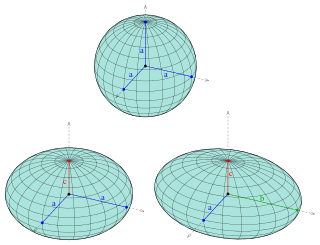
An ellipsoid is a surface that may be obtained from a sphere by deforming it by means of directional scalings, or more generally, of an affine transformation.

In mechanics and geometry, the 3D rotation group, often denoted SO(3), is the group of all rotations about the origin of three-dimensional Euclidean space under the operation of composition.

Fourier optics is the study of classical optics using Fourier transforms (FTs), in which the waveform being considered is regarded as made up of a combination, or superposition, of plane waves. It has some parallels to the Huygens–Fresnel principle, in which the wavefront is regarded as being made up of a combination of spherical wavefronts whose sum is the wavefront being studied. A key difference is that Fourier optics considers the plane waves to be natural modes of the propagation medium, as opposed to Huygens–Fresnel, where the spherical waves originate in the physical medium.

<span class="mw-page-title-main">3D projection</span> Design technique

A 3D projection is a design technique used to display a three-dimensional (3D) object on a two-dimensional (2D) surface. These projections rely on visual perspective and aspect analysis to project a complex object for viewing capability on a simpler plane.

<span class="mw-page-title-main">Cone</span> Geometric shape

A cone is a three-dimensional geometric shape that tapers smoothly from a flat base to a point called the apex or vertex.

In optics, the Fraunhofer diffraction equation is used to model the diffraction of waves when plane waves are incident on a diffracting object, and the diffraction pattern is viewed at a sufficiently long distance from the object, and also when it is viewed at the focal plane of an imaging lens. In contrast, the diffraction pattern created near the diffracting object is given by the Fresnel diffraction equation.

<span class="mw-page-title-main">Cissoid of Diocles</span> Cubic plane curve

In geometry, the cissoid of Diocles is a cubic plane curve notable for the property that it can be used to construct two mean proportionals to a given ratio. In particular, it can be used to double a cube. It can be defined as the cissoid of a circle and a line tangent to it with respect to the point on the circle opposite to the point of tangency. In fact, the curve family of cissoids is named for this example and some authors refer to it simply as the cissoid. It has a single cusp at the pole, and is symmetric about the diameter of the circle which is the line of tangency of the cusp. The line is an asymptote. It is a member of the conchoid of de Sluze family of curves and in form it resembles a tractrix.

<span class="mw-page-title-main">Pedal curve</span> Curve generated by the projections of a fixed point on the tangents of another curve

In mathematics, a pedal curve of a given curve results from the orthogonal projection of a fixed point on the tangent lines of this curve. More precisely, for a plane curve C and a given fixed pedal pointP, the pedal curve of C is the locus of points X so that the line PX is perpendicular to a tangent T to the curve passing through the point X. Conversely, at any point R on the curve C, let T be the tangent line at that point R; then there is a unique point X on the tangent T which forms with the pedal point P a line perpendicular to the tangent T – the pedal curve is the set of such points X, called the foot of the perpendicular to the tangent T from the fixed point P, as the variable point R ranges over the curve C.

<span class="mw-page-title-main">Strophoid</span> Geometric curve constructed from another curve and two points

In geometry, a strophoid is a curve generated from a given curve C and points A and O as follows: Let L be a variable line passing through O and intersecting C at K. Now let P1 and P2 be the two points on L whose distance from K is the same as the distance from A to K. The locus of such points P1 and P2 is then the strophoid of C with respect to the pole O and fixed point A. Note that AP1 and AP2 are at right angles in this construction.

Photon polarization is the quantum mechanical description of the classical polarized sinusoidal plane electromagnetic wave. An individual photon can be described as having right or left circular polarization, or a superposition of the two. Equivalently, a photon can be described as having horizontal or vertical linear polarization, or a superposition of the two.

In geometry, various formalisms exist to express a rotation in three dimensions as a mathematical transformation. In physics, this concept is applied to classical mechanics where rotational kinematics is the science of quantitative description of a purely rotational motion. The orientation of an object at a given instant is described with the same tools, as it is defined as an imaginary rotation from a reference placement in space, rather than an actually observed rotation from a previous placement in space.

There are several equivalent ways for defining trigonometric functions, and the proof of the trigonometric identities between them depend on the chosen definition. The oldest and somehow the most elementary definition is based on the geometry of right triangles. The proofs given in this article use this definition, and thus apply to non-negative angles not greater than a right angle. For greater and negative angles, see Trigonometric functions.

<span class="mw-page-title-main">Range of a projectile</span>

In physics, a projectile launched with specific initial conditions will have a range. It may be more predictable assuming a flat Earth with a uniform gravity field, and no air resistance.

<span class="mw-page-title-main">Gravitational lensing formalism</span>

In general relativity, a point mass deflects a light ray with impact parameter by an angle approximately equal to

<span class="mw-page-title-main">Kepler orbit</span> Celestial orbit whose trajectory is a conic section in the orbital plane

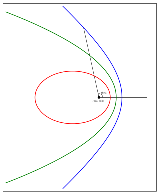
In celestial mechanics, a Kepler orbit is the motion of one body relative to another, as an ellipse, parabola, or hyperbola, which forms a two-dimensional orbital plane in three-dimensional space. A Kepler orbit can also form a straight line. It considers only the point-like gravitational attraction of two bodies, neglecting perturbations due to gravitational interactions with other objects, atmospheric drag, solar radiation pressure, a non-spherical central body, and so on. It is thus said to be a solution of a special case of the two-body problem, known as the Kepler problem. As a theory in classical mechanics, it also does not take into account the effects of general relativity. Keplerian orbits can be parametrized into six orbital elements in various ways.

References