Simpson's paradox

Last updated
Simpson's paradox for quantitative data: a positive trend ( ,  ) appears for two separate groups, whereas a negative trend ( ) appears when the groups are combined. Simpson's paradox continuous.svg
Simpson's paradox for quantitative data: a positive trend ( ,  ) appears for two separate groups, whereas a negative trend ( ) appears when the groups are combined.
Visualization of Simpson's paradox on data resembling real-world variability indicates that risk of misjudgment of true causal relationship can be hard to spot. Simpsons paradox - animation.gif
Visualization of Simpson's paradox on data resembling real-world variability indicates that risk of misjudgment of true causal relationship can be hard to spot.

Simpson's paradox is a phenomenon in probability and statistics in which a trend appears in several groups of data but disappears or reverses when the groups are combined. This result is often encountered in social-science and medical-science statistics, [1] [2] [3] and is particularly problematic when frequency data are unduly given causal interpretations. [4] The paradox can be resolved when confounding variables and causal relations are appropriately addressed in the statistical modeling [4] [5] (e.g., through cluster analysis [6] ).

Contents

Simpson's paradox has been used to illustrate the kind of misleading results that the misuse of statistics can generate. [7] [8]

Edward H. Simpson first described this phenomenon in a technical paper in 1951, [9] but the statisticians Karl Pearson (in 1899 [10] ) and Udny Yule (in 1903 [11] ) had mentioned similar effects earlier. The name Simpson's paradox was introduced by Colin R. Blyth in 1972. [12] It is also referred to as Simpson's reversal, the Yule–Simpson effect, the amalgamation paradox, or the reversal paradox. [13]

Mathematician Jordan Ellenberg argues that Simpson's paradox is misnamed as "there's no contradiction involved, just two different ways to think about the same data" and suggests that its lesson "isn't really to tell us which viewpoint to take but to insist that we keep both the parts and the whole in mind at once." [14]

Examples

UC Berkeley gender bias

One of the best-known examples of Simpson's paradox comes from a study of gender bias among graduate school admissions to University of California, Berkeley. The admission figures for the fall of 1973 showed that men applying were more likely than women to be admitted, and the difference was so large that it was unlikely to be due to chance. [15] [16]

AllMenWomen
ApplicantsAdmittedApplicantsAdmittedApplicantsAdmitted
Total12,76341%8,44244%4,32135%

However, when taking into account the information about departments being applied to, the different rejection percentages reveal the different difficulty of getting into the department, and at the same time it showed that women tended to apply to more competitive departments with lower rates of admission, even among qualified applicants (such as in the English department), whereas men tended to apply to less competitive departments with higher rates of admission (such as in the engineering department). The pooled and corrected data showed a "small but statistically significant bias in favor of women". [16]

The data from the six largest departments are listed below:

DepartmentAllMenWomen
ApplicantsAdmittedApplicantsAdmittedApplicantsAdmitted
A93364%82562%10882%
B58563%56063%2568%
C91835%32537%59334%
D79234%41733%37535%
E58425%19128%39324%
F7146%3736%3417%
Total452639%269145%183530%

Legend:

  greater percentage of successful applicants than the other gender
  greater number of applicants than the other gender

bold - the two 'most applied for' departments for each gender

The entire data showed total of 4 out of 85 departments to be significantly biased against women, while 6 to be significantly biased against men (not all present in the 'six largest departments' table above). Notably, the numbers of biased departments were not the basis for the conclusion, but rather it was the gender admissions pooled across all departments, while weighing by each department's rejection rate across all of its applicants. [16]

Kidney stone treatment

Another example comes from a real-life medical study [17] comparing the success rates of two treatments for kidney stones. [18] The table below shows the success rates (the term success rate here actually means the success proportion) and numbers of treatments for treatments involving both small and large kidney stones, where Treatment A includes open surgical procedures and Treatment B includes closed surgical procedures. The numbers in parentheses indicate the number of success cases over the total size of the group.

Treatment
Stone size   
Treatment ATreatment B
Small stonesGroup 1
93% (81/87)
Group 2
87% (234/270)
Large stonesGroup 3
73% (192/263)
Group 4
69% (55/80)
Both78% (273/350)83% (289/350)

The paradoxical conclusion is that treatment A is more effective when used on small stones, and also when used on large stones, yet treatment B appears to be more effective when considering both sizes at the same time. In this example, the "lurking" variable (or confounding variable) causing the paradox is the size of the stones, which was not previously known to researchers to be important until its effects were included.[ citation needed ]

Which treatment is considered better is determined by which success ratio (successes/total) is larger. The reversal of the inequality between the two ratios when considering the combined data, which creates Simpson's paradox, happens because two effects occur together:[ citation needed ]

  1. The sizes of the groups, which are combined when the lurking variable is ignored, are very different. Doctors tend to give cases with large stones the better treatment A, and the cases with small stones the inferior treatment B. Therefore, the totals are dominated by groups 3 and 2, and not by the two much smaller groups 1 and 4.
  2. The lurking variable, stone size, has a large effect on the ratios; i.e., the success rate is more strongly influenced by the severity of the case than by the choice of treatment. Therefore, the group of patients with large stones using treatment A (group 3) does worse than the group with small stones, even if the latter used the inferior treatment B (group 2).

Based on these effects, the paradoxical result is seen to arise because the effect of the size of the stones overwhelms the benefits of the better treatment (A). In short, the less effective treatment B appeared to be more effective because it was applied more frequently to the small stones cases, which were easier to treat. [18]

Batting averages

A common example of Simpson's paradox involves the batting averages of players in professional baseball. It is possible for one player to have a higher batting average than another player each year for a number of years, but to have a lower batting average across all of those years. This phenomenon can occur when there are large differences in the number of at bats between the years. Mathematician Ken Ross demonstrated this using the batting average of two baseball players, Derek Jeter and David Justice, during the years 1995 and 1996: [19] [20]

Year
Batter  
19951996Combined
Derek Jeter12/48.250183/582.314195/630.310
David Justice104/411.25345/140.321149/551.270

In both 1995 and 1996, Justice had a higher batting average (in bold type) than Jeter did. However, when the two baseball seasons are combined, Jeter shows a higher batting average than Justice. According to Ross, this phenomenon would be observed about once per year among the possible pairs of players. [19]

Vector interpretation

Vector interpretation of Simpson's paradox Simpson paradox vectors.svg
Vector interpretation of Simpson's paradox

Simpson's paradox can also be illustrated using a 2-dimensional vector space. [21] A success rate of (i.e., successes/attempts) can be represented by a vector , with a slope of . A steeper vector then represents a greater success rate. If two rates and are combined, as in the examples given above, the result can be represented by the sum of the vectors and , which according to the parallelogram rule is the vector , with slope .

Simpson's paradox says that even if a vector (in orange in figure) has a smaller slope than another vector (in blue), and has a smaller slope than , the sum of the two vectors can potentially still have a larger slope than the sum of the two vectors , as shown in the example. For this to occur one of the orange vectors must have a greater slope than one of the blue vectors (here and ), and these will generally be longer than the alternatively subscripted vectors – thereby dominating the overall comparison.

Correlation between variables

Simpson's reversal can also arise in correlations, in which two variables appear to have (say) a positive correlation towards one another, when in fact they have a negative correlation, the reversal having been brought about by a "lurking" confounder. Berman et al. [22] give an example from economics, where a dataset suggests overall demand is positively correlated with price (that is, higher prices lead to more demand), in contradiction of expectation. Analysis reveals time to be the confounding variable: plotting both price and demand against time reveals the expected negative correlation over various periods, which then reverses to become positive if the influence of time is ignored by simply plotting demand against price.

Psychology

Psychological interest in Simpson's paradox seeks to explain why people deem sign reversal to be impossible at first. The question is where people get this strong intuition from, and how it is encoded in the mind.

Simpson's paradox demonstrates that this intuition cannot be derived from either classical logic or probability calculus alone, and thus led philosophers to speculate that it is supported by an innate causal logic that guides people in reasoning about actions and their consequences. [4] Savage's sure-thing principle [12] is an example of what such logic may entail. A qualified version of Savage's sure thing principle can indeed be derived from Pearl's do-calculus [4] and reads: "An action A that increases the probability of an event B in each subpopulation Ci of C must also increase the probability of B in the population as a whole, provided that the action does not change the distribution of the subpopulations." This suggests that knowledge about actions and consequences is stored in a form resembling Causal Bayesian Networks.

Probability

A paper by Pavlides and Perlman presents a proof, due to Hadjicostas, that in a random 2 × 2 × 2 table with uniform distribution, Simpson's paradox will occur with a probability of exactly 160. [23] A study by Kock suggests that the probability that Simpson's paradox would occur at random in path models (i.e., models generated by path analysis) with two predictors and one criterion variable is approximately 12.8 percent; slightly higher than 1 occurrence per 8 path models. [24]

Simpson's second paradox

A second, less well-known paradox was also discussed in Simpson's 1951 paper. It can occur when the "sensible interpretation" is not necessarily found in the separated data, like in the Kidney Stone example, but can instead reside in the combined data. Whether the partitioned or combined form of the data should be used hinges on the process giving rise to the data, meaning the correct interpretation of the data cannot always be determined by simply observing the tables. [25]

Judea Pearl has shown that, in order for the partitioned data to represent the correct causal relationships between any two variables, and , the partitioning variables must satisfy a graphical condition called "back-door criterion": [26] [27]

  1. They must block all spurious paths between and
  2. No variable can be affected by

This criterion provides an algorithmic solution to Simpson's second paradox, and explains why the correct interpretation cannot be determined by data alone; two different graphs, both compatible with the data, may dictate two different back-door criteria.

When the back-door criterion is satisfied by a set Z of covariates, the adjustment formula (see Confounding) gives the correct causal effect of X on Y. If no such set exists, Pearl's do-calculus can be invoked to discover other ways of estimating the causal effect. [4] [28] The completeness of do-calculus [29] [28] can be viewed as offering a complete resolution of the Simpson's paradox.

Criticism

One criticism is that the paradox is not really a paradox at all, but rather a failure to properly account for confounding variables or to consider causal relationships between variables. [30]

Another criticism of the apparent Simpson's paradox is that it may be a result of the specific way that data is stratified or grouped. The phenomenon may disappear or even reverse if the data is stratified differently or if different confounding variables are considered. Simpson's example actually highlighted a phenomenon called noncollapsibility, [31] which occurs when subgroups with high proportions do not make simple averages when combined. This suggests that the paradox may not be a universal phenomenon, but rather a specific instance of a more general statistical issue.

Critics of the apparent Simpson's paradox also argue that the focus on the paradox may distract from more important statistical issues, such as the need for careful consideration of confounding variables and causal relationships when interpreting data. [32]

Despite these criticisms, the apparent Simpson's paradox remains a popular and intriguing topic in statistics and data analysis. It continues to be studied and debated by researchers and practitioners in a wide range of fields, and it serves as a valuable reminder of the importance of careful statistical analysis and the potential pitfalls of simplistic interpretations of data.

See also

Related Research Articles

Bell's theorem is a term encompassing a number of closely related results in physics, all of which determine that quantum mechanics is incompatible with local hidden-variable theories, given some basic assumptions about the nature of measurement. "Local" here refers to the principle of locality, the idea that a particle can only be influenced by its immediate surroundings, and that interactions mediated by physical fields cannot propagate faster than the speed of light. "Hidden variables" are putative properties of quantum particles that are not included in quantum theory but nevertheless affect the outcome of experiments. In the words of physicist John Stewart Bell, for whom this family of results is named, "If [a hidden-variable theory] is local it will not agree with quantum mechanics, and if it agrees with quantum mechanics it will not be local."

An odds ratio (OR) is a statistic that quantifies the strength of the association between two events, A and B. The odds ratio is defined as the ratio of the odds of A in the presence of B and the odds of A in the absence of B, or equivalently, the ratio of the odds of B in the presence of A and the odds of B in the absence of A. Two events are independent if and only if the OR equals 1, i.e., the odds of one event are the same in either the presence or absence of the other event. If the OR is greater than 1, then A and B are associated (correlated) in the sense that, compared to the absence of B, the presence of B raises the odds of A, and symmetrically the presence of A raises the odds of B. Conversely, if the OR is less than 1, then A and B are negatively correlated, and the presence of one event reduces the odds of the other event.

<span class="mw-page-title-main">Spurious relationship</span> Apparent, but false, correlation between causally-independent variables

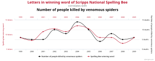
In statistics, a spurious relationship or spurious correlation is a mathematical relationship in which two or more events or variables are associated but not causally related, due to either coincidence or the presence of a certain third, unseen factor.

<span class="mw-page-title-main">Data dredging</span> Misuse of data analysis

Data dredging is the misuse of data analysis to find patterns in data that can be presented as statistically significant, thus dramatically increasing and understating the risk of false positives. This is done by performing many statistical tests on the data and only reporting those that come back with significant results.

Linear discriminant analysis (LDA), normal discriminant analysis (NDA), or discriminant function analysis is a generalization of Fisher's linear discriminant, a method used in statistics and other fields, to find a linear combination of features that characterizes or separates two or more classes of objects or events. The resulting combination may be used as a linear classifier, or, more commonly, for dimensionality reduction before later classification.

In statistics, econometrics, epidemiology and related disciplines, the method of instrumental variables (IV) is used to estimate causal relationships when controlled experiments are not feasible or when a treatment is not successfully delivered to every unit in a randomized experiment. Intuitively, IVs are used when an explanatory variable of interest is correlated with the error term (endogenous), in which case ordinary least squares and ANOVA give biased results. A valid instrument induces changes in the explanatory variable but has no independent effect on the dependent variable and is not correlated with the error term, allowing a researcher to uncover the causal effect of the explanatory variable on the dependent variable.

<span class="mw-page-title-main">Granger causality</span> Statistical hypothesis test for forecasting

The Granger causality test is a statistical hypothesis test for determining whether one time series is useful in forecasting another, first proposed in 1969. Ordinarily, regressions reflect "mere" correlations, but Clive Granger argued that causality in economics could be tested for by measuring the ability to predict the future values of a time series using prior values of another time series. Since the question of "true causality" is deeply philosophical, and because of the post hoc ergo propter hoc fallacy of assuming that one thing preceding another can be used as a proof of causation, econometricians assert that the Granger test finds only "predictive causality". Using the term "causality" alone is a misnomer, as Granger-causality is better described as "precedence", or, as Granger himself later claimed in 1977, "temporally related". Rather than testing whether Xcauses Y, the Granger causality tests whether X forecastsY.

This glossary of statistics and probability is a list of definitions of terms and concepts used in the mathematical sciences of statistics and probability, their sub-disciplines, and related fields. For additional related terms, see Glossary of mathematics and Glossary of experimental design.

<span class="mw-page-title-main">Confounding</span> Variable or factor in causal inference

In causal inference, a confounder is a variable that influences both the dependent variable and independent variable, causing a spurious association. Confounding is a causal concept, and as such, cannot be described in terms of correlations or associations. The existence of confounders is an important quantitative explanation why correlation does not imply causation. Some notations are explicitly designed to identify the existence, possible existence, or non-existence of confounders in causal relationships between elements of a system.

In information theory, information dimension is an information measure for random vectors in Euclidean space, based on the normalized entropy of finely quantized versions of the random vectors. This concept was first introduced by Alfréd Rényi in 1959.

<span class="mw-page-title-main">Causal model</span> Conceptual model in philosophy of science

In the philosophy of science, a causal model is a conceptual model that describes the causal mechanisms of a system. Several types of causal notation may be used in the development of a causal model. Causal models can improve study designs by providing clear rules for deciding which independent variables need to be included/controlled for.

In the statistical analysis of observational data, propensity score matching (PSM) is a statistical matching technique that attempts to estimate the effect of a treatment, policy, or other intervention by accounting for the covariates that predict receiving the treatment. PSM attempts to reduce the bias due to confounding variables that could be found in an estimate of the treatment effect obtained from simply comparing outcomes among units that received the treatment versus those that did not. Paul R. Rosenbaum and Donald Rubin introduced the technique in 1983.

<span class="mw-page-title-main">Plot (graphics)</span> Graphical technique for data sets

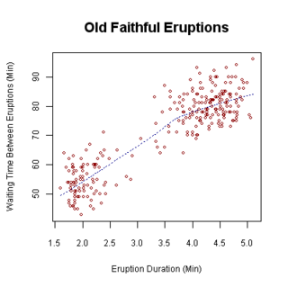
A plot is a graphical technique for representing a data set, usually as a graph showing the relationship between two or more variables. The plot can be drawn by hand or by a computer. In the past, sometimes mechanical or electronic plotters were used. Graphs are a visual representation of the relationship between variables, which are very useful for humans who can then quickly derive an understanding which may not have come from lists of values. Given a scale or ruler, graphs can also be used to read off the value of an unknown variable plotted as a function of a known one, but this can also be done with data presented in tabular form. Graphs of functions are used in mathematics, sciences, engineering, technology, finance, and other areas.

Isoline retrieval is a remote sensing inverse method that retrieves one or more isolines of a trace atmospheric constituent or variable. When used to validate another contour, it is the most accurate method possible for the task. When used to retrieve a whole field, it is a general, nonlinear inverse method and a robust estimator.

<span class="mw-page-title-main">Collider (statistics)</span> Variable that is causally influenced by two or more variables

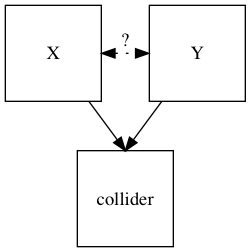
In statistics and causal graphs, a variable is a collider when it is causally influenced by two or more variables. The name "collider" reflects the fact that in graphical models, the arrow heads from variables that lead into the collider appear to "collide" on the node that is the collider. They are sometimes also referred to as inverted forks.

Causal inference is the process of determining the independent, actual effect of a particular phenomenon that is a component of a larger system. The main difference between causal inference and inference of association is that causal inference analyzes the response of an effect variable when a cause of the effect variable is changed. The study of why things occur is called etiology, and can be described using the language of scientific causal notation. Causal inference is said to provide the evidence of causality theorized by causal reasoning.

In statistics, Lord's paradox raises the issue of when it is appropriate to control for baseline status. In three papers, Frederic M. Lord gave examples when statisticians could reach different conclusions depending on whether they adjust for pre-existing differences. Holland & Rubin (1983) use these examples to illustrate how there may be multiple valid descriptive comparisons in the data, but causal conclusions require an underlying (untestable) causal model. Pearl used these examples to illustrate how graphical causal models resolve the issue of when control for baseline status is appropriate.

In statistics, econometrics, epidemiology, genetics and related disciplines, causal graphs are probabilistic graphical models used to encode assumptions about the data-generating process.

In statistics, linear regression is a statistical model which estimates the linear relationship between a scalar response and one or more explanatory variables. The case of one explanatory variable is called simple linear regression; for more than one, the process is called multiple linear regression. This term is distinct from multivariate linear regression, where multiple correlated dependent variables are predicted, rather than a single scalar variable. If the explanatory variables are measured with error then errors-in-variables models are required, also known as measurement error models.

Fairness in machine learning refers to the various attempts at correcting algorithmic bias in automated decision processes based on machine learning models. Decisions made by computers after a machine-learning process may be considered unfair if they were based on variables considered sensitive. For example gender, ethnicity, sexual orientation or disability. As it is the case with many ethical concepts, definitions of fairness and bias are always controversial. In general, fairness and bias are considered relevant when the decision process impacts people's lives. In machine learning, the problem of algorithmic bias is well known and well studied. Outcomes may be skewed by a range of factors and thus might be considered unfair with respect to certain groups or individuals. An example would be the way social media sites deliver personalized news to consumers.

References

  1. Clifford H. Wagner (February 1982). "Simpson's Paradox in Real Life". The American Statistician . 36 (1): 46–48. doi:10.2307/2684093. JSTOR   2684093.
  2. Holt, G. B. (2016). Potential Simpson's paradox in multicenter study of intraperitoneal chemotherapy for ovarian cancer. Journal of Clinical Oncology, 34(9), 1016–1016.
  3. Franks, Alexander; Airoldi, Edoardo; Slavov, Nikolai (2017). "Post-transcriptional regulation across human tissues". PLOS Computational Biology. 13 (5): e1005535. arXiv: 1506.00219 . Bibcode:2017PLSCB..13E5535F. doi: 10.1371/journal.pcbi.1005535 . ISSN   1553-7358. PMC   5440056 . PMID   28481885.
  4. 1 2 3 4 5 Judea Pearl. Causality: Models, Reasoning, and Inference, Cambridge University Press (2000, 2nd edition 2009). ISBN   0-521-77362-8.
  5. Kock, N., & Gaskins, L. (2016). Simpson's paradox, moderation and the emergence of quadratic relationships in path models: An information systems illustration. International Journal of Applied Nonlinear Science, 2(3), 200–234.
  6. Rogier A. Kievit, Willem E. Frankenhuis, Lourens J. Waldorp and Denny Borsboom, Simpson's paradox in psychological science: a practical guide https://doi.org/10.3389/fpsyg.2013.00513
  7. Robert L. Wardrop (February 1995). "Simpson's Paradox and the Hot Hand in Basketball". The American Statistician, 49 (1): pp. 24–28.
  8. Alan Agresti (2002). "Categorical Data Analysis" (Second edition). John Wiley and Sons ISBN   0-471-36093-7
  9. Simpson, Edward H. (1951). "The Interpretation of Interaction in Contingency Tables". Journal of the Royal Statistical Society, Series B. 13: 238–241.
  10. Pearson, Karl; Lee, Alice; Bramley-Moore, Lesley (1899). "Genetic (reproductive) selection: Inheritance of fertility in man, and of fecundity in thoroughbred racehorses". Philosophical Transactions of the Royal Society A . 192: 257–330. doi: 10.1098/rsta.1899.0006 .
  11. G. U. Yule (1903). "Notes on the Theory of Association of Attributes in Statistics". Biometrika . 2 (2): 121–134. doi:10.1093/biomet/2.2.121.
  12. 1 2 Colin R. Blyth (June 1972). "On Simpson's Paradox and the Sure-Thing Principle". Journal of the American Statistical Association. 67 (338): 364–366. doi:10.2307/2284382. JSTOR   2284382.
  13. I. J. Good, Y. Mittal (June 1987). "The Amalgamation and Geometry of Two-by-Two Contingency Tables". The Annals of Statistics . 15 (2): 694–711. doi: 10.1214/aos/1176350369 . ISSN   0090-5364. JSTOR   2241334.
  14. Ellenberg, Jordan (May 25, 2021). Shape: The Hidden Geometry of Information, Biology, Strategy, Democracy and Everything Else. New York: Penguin Press. p. 228. ISBN   978-1-9848-7905-9. OCLC   1226171979.
  15. David Freedman, Robert Pisani, and Roger Purves (2007), Statistics (4th edition), W. W. Norton. ISBN   0-393-92972-8.
  16. 1 2 3 P.J. Bickel, E.A. Hammel and J.W. O'Connell (1975). "Sex Bias in Graduate Admissions: Data From Berkeley" (PDF). Science . 187 (4175): 398–404. Bibcode:1975Sci...187..398B. doi:10.1126/science.187.4175.398. PMID   17835295. S2CID   15278703. Archived (PDF) from the original on 2016-06-04.
  17. C. R. Charig; D. R. Webb; S. R. Payne; J. E. Wickham (29 March 1986). "Comparison of treatment of renal calculi by open surgery, percutaneous nephrolithotomy, and extracorporeal shockwave lithotripsy". Br Med J (Clin Res Ed) . 292 (6524): 879–882. doi:10.1136/bmj.292.6524.879. PMC   1339981 . PMID   3083922.
  18. 1 2 Steven A. Julious; Mark A. Mullee (3 December 1994). "Confounding and Simpson's paradox". BMJ . 309 (6967): 1480–1481. doi:10.1136/bmj.309.6967.1480. PMC   2541623 . PMID   7804052.
  19. 1 2 Ken Ross. "A Mathematician at the Ballpark: Odds and Probabilities for Baseball Fans (Paperback)" Pi Press, 2004. ISBN   0-13-147990-3. 12–13
  20. Statistics available from Baseball-Reference.com: Data for Derek Jeter; Data for David Justice.
  21. Kocik Jerzy (2001). "Proofs without Words: Simpson's Paradox" (PDF). Mathematics Magazine . 74 (5): 399. doi:10.2307/2691038. JSTOR   2691038. Archived (PDF) from the original on 2010-06-12.
  22. Berman, S. DalleMule, L. Greene, M., Lucker, J. (2012), "Simpson's Paradox: A Cautionary Tale in Advanced Analytics Archived 2020-05-10 at the Wayback Machine ", Significance .
  23. Marios G. Pavlides & Michael D. Perlman (August 2009). "How Likely is Simpson's Paradox?". The American Statistician . 63 (3): 226–233. doi:10.1198/tast.2009.09007. S2CID   17481510.
  24. Kock, N. (2015). How likely is Simpson's paradox in path models? International Journal of e-Collaboration, 11(1), 1–7.
  25. Norton, H. James; Divine, George (August 2015). "Simpson's paradox ... and how to avoid it". Significance. 12 (4): 40–43. doi: 10.1111/j.1740-9713.2015.00844.x .
  26. Pearl, Judea (2014). "Understanding Simpson's Paradox". The American Statistician. 68 (1): 8–13. doi:10.2139/ssrn.2343788. S2CID   2626833.
  27. Pearl, Judea (1993). "Graphical Models, Causality, and Intervention". Statistical Science. 8 (3): 266–269. doi: 10.1214/ss/1177010894 .
  28. 1 2 Pearl, J.; Mackenzie, D. (2018). The Book of Why: The New Science of Cause and Effect. New York, NY: Basic Books.
  29. Shpitser, I.; Pearl, J. (2006). Dechter, R.; Richardson, T.S. (eds.). "Identification of Conditional Interventional Distributions". Proceedings of the Twenty-Second Conference on Uncertainty in Artificial Intelligence. Corvallis, OR: AUAI Press: 437–444.
  30. Blyth, Colin R. (June 1972). "On Simpson's Paradox and the Sure-Thing Principle". Journal of the American Statistical Association. 67 (338): 364–366. doi:10.1080/01621459.1972.10482387. ISSN   0162-1459.
  31. Greenland, Sander (2021-11-01). "Noncollapsibility, confounding, and sparse-data bias. Part 2: What should researchers make of persistent controversies about the odds ratio?". Journal of Clinical Epidemiology. 139: 264–268. doi: 10.1016/j.jclinepi.2021.06.004 . ISSN   0895-4356. PMID   34119647.
  32. Hernán, Miguel A.; Clayton, David; Keiding, Niels (June 2011). "The Simpson's paradox unraveled". International Journal of Epidemiology. 40 (3): 780–785. doi:10.1093/ije/dyr041. ISSN   1464-3685. PMC   3147074 . PMID   21454324.

Bibliography