Aliasing

Last updated

An example of aliasing
Moire pattern of bricks.jpg
This full-sized image shows what a properly sampled image of a brick wall should look like with a screen of sufficient resolution.
Moire pattern of bricks small.jpg
When the resolution is reduced, aliasing appears in the form of a moiré pattern.
WagonWheelEffect.gif
The motion of the 'camera' at a constant shutter speed creates temporal aliasing known as the wagon wheel effect. The speed of the "camera", moving towards the right, constantly increases at the same rate with the objects sliding to the left. Halfway through the 24-second loop, the objects appear to suddenly shift and head in the reverse direction, towards the right.

In signal processing and related disciplines, aliasing is the overlapping of frequency components resulting from a sample rate below the Nyquist rate. This overlap results in distortion or artifacts when the signal is reconstructed from samples which causes the reconstructed signal to differ from the original continuous signal. Aliasing that occurs in signals sampled in time, for instance in digital audio or the stroboscopic effect, is referred to as temporal aliasing. Aliasing in spatially sampled signals (e.g., moiré patterns in digital images) is referred to as spatial aliasing.

Contents

Aliasing is generally avoided by applying low-pass filters or anti-aliasing filters (AAF) to the input signal before sampling and when converting a signal from a higher to a lower sampling rate. Suitable reconstruction filtering should then be used when restoring the sampled signal to the continuous domain or converting a signal from a lower to a higher sampling rate. For spatial anti-aliasing, the types of anti-aliasing include fast approximate anti-aliasing (FXAA), multisample anti-aliasing, and supersampling.

Description

Dots in the sky due to spatial aliasing caused by halftone resized to a lower resolution Risingstar test crop.png
Dots in the sky due to spatial aliasing caused by halftone resized to a lower resolution

When a digital image is viewed, a reconstruction is performed by a display or printer device, and by the eyes and the brain. If the image data is processed incorrectly during sampling or reconstruction, the reconstructed image will differ from the original image, and an alias is seen.

An example of spatial aliasing is the moiré pattern observed in a poorly pixelized image of a brick wall. Spatial anti-aliasing techniques avoid such poor pixelizations. Aliasing can be caused either by the sampling stage or the reconstruction stage; these may be distinguished by calling sampling aliasing prealiasing and reconstruction aliasing postaliasing. [1]

Temporal aliasing is a major concern in the sampling of video and audio signals. Music, for instance, may contain high-frequency components that are inaudible to humans. If a piece of music is sampled at 32,000 samples per second (Hz), any frequency components at or above 16,000 Hz (the Nyquist frequency for this sampling rate) will cause aliasing when the music is reproduced by a digital-to-analog converter (DAC). The high frequencies in the analog signal will appear as lower frequencies (wrong alias) in the recorded digital sample and, hence, cannot be reproduced by the DAC. To prevent this, an anti-aliasing filter is used to remove components above the Nyquist frequency prior to sampling.

In video or cinematography, temporal aliasing results from the limited frame rate, and causes the wagon-wheel effect, whereby a spoked wheel appears to rotate too slowly or even backwards. Aliasing has changed its apparent frequency of rotation. A reversal of direction can be described as a negative frequency. Temporal aliasing frequencies in video and cinematography are determined by the frame rate of the camera, but the relative intensity of the aliased frequencies is determined by the shutter timing (exposure time) or the use of a temporal aliasing reduction filter during filming. [2] [ unreliable source? ]

Like the video camera, most sampling schemes are periodic; that is, they have a characteristic sampling frequency in time or in space. Digital cameras provide a certain number of samples (pixels) per degree or per radian, or samples per mm in the focal plane of the camera. Audio signals are sampled (digitized) with an analog-to-digital converter, which produces a constant number of samples per second. Some of the most dramatic and subtle examples of aliasing occur when the signal being sampled also has periodic content.

Bandlimited functions

Actual signals have a finite duration and their frequency content, as defined by the Fourier transform, has no upper bound. Some amount of aliasing always occurs when such functions are sampled. Functions whose frequency content is bounded (bandlimited) have an infinite duration in the time domain. If sampled at a high enough rate, determined by the bandwidth, the original function can, in theory, be perfectly reconstructed from the infinite set of samples.

Bandpass signals

Sometimes aliasing is used intentionally on signals with no low-frequency content, called bandpass signals. Undersampling, which creates low-frequency aliases, can produce the same result, with less effort, as frequency-shifting the signal to lower frequencies before sampling at the lower rate. Some digital channelizers exploit aliasing in this way for computational efficiency. [3]   (See Sampling (signal processing), Nyquist rate (relative to sampling), and Filter bank.)

Sampling sinusoidal functions

Fig.2 Upper left: Animation depicts a sequence of sinusoids, each with a higher frequency than the previous ones. These "true" signals are also being sampled (blue dots) at a constant frequency/rate,
f
s
.
{\displaystyle f_{s}.}

Upper right: The
continuous
Fourier transform of the sinusoid (not the samples). The single non-zero component, depicting the actual frequency, means there is no ambiguity.
Lower right: The
discrete
Fourier transform of just the available samples. The presence of two components means the samples can fit at least two different sinusoids, one of which is the true frequency (upper-right).
Lower left: Using the same samples (now in orange), the default reconstruction algorithm produces the lower-frequency sinusoid. FFT aliasing 600.gif
Fig.2 Upper left: Animation depicts a sequence of sinusoids, each with a higher frequency than the previous ones. These "true" signals are also being sampled (blue dots) at a constant frequency/rate,
Upper right: The continuous Fourier transform of the sinusoid (not the samples). The single non-zero component, depicting the actual frequency, means there is no ambiguity.
Lower right: The discrete Fourier transform of just the available samples. The presence of two components means the samples can fit at least two different sinusoids, one of which is the true frequency (upper-right).
Lower left: Using the same samples (now in orange), the default reconstruction algorithm produces the lower-frequency sinusoid.

Sinusoids are an important type of periodic function, because realistic signals are often modeled as the summation of many sinusoids of different frequencies and different amplitudes (for example, with a Fourier series or transform). Understanding what aliasing does to the individual sinusoids is useful in understanding what happens to their sum.

When sampling a function at frequency fs (intervals 1/fs), the following functions of time (t) yield identical sets of samples: {sin(2π( f+Nfs) t + φ), N = 0, ±1, ±2, ±3,...}. A frequency spectrum of the samples produces equally strong responses at all those frequencies. Without collateral information, the frequency of the original function is ambiguous. So the functions and their frequencies are said to be aliases of each other. Noting the trigonometric identity:

we can write all the alias frequencies as positive values: . For example, a snapshot of the lower right frame of Fig.2 shows a component at the actual frequency and another component at alias . As increases during the animation, decreases. The point at which they are equal is an axis of symmetry called the folding frequency, also known as Nyquist frequency .

Aliasing matters when one attempts to reconstruct the original waveform from its samples. The most common reconstruction technique produces the smallest of the frequencies. So it is usually important that be the unique minimum.  A necessary and sufficient condition for that is called the Nyquist condition. The lower left frame of Fig.2 depicts the typical reconstruction result of the available samples. Until exceeds the Nyquist frequency, the reconstruction matches the actual waveform (upper left frame). After that, it is the low frequency alias of the upper frame.

Folding

The figures below offer additional depictions of aliasing, due to sampling. A graph of amplitude vs frequency (not time) for a single sinusoid at frequency  0.6 fs  and some of its aliases at  0.4 fs, 1.4 fs,  and  1.6 fs  would look like the 4 black dots in Fig.3. The red lines depict the paths (loci) of the 4 dots if we were to adjust the frequency and amplitude of the sinusoid along the solid red segment (between  fs/2  and  fs).  No matter what function we choose to change the amplitude vs frequency, the graph will exhibit symmetry between 0 and  fs.  Folding is often observed in practice when viewing the frequency spectrum of real-valued samples, such as Fig.4..

Fig.3: The black dots are aliases of each other. The solid red line is an
example
of amplitude varying with frequency. The dashed red lines are the corresponding paths of the aliases. Aliasing-folding SVG.svg
Fig.3: The black dots are aliases of each other. The solid red line is an example of amplitude varying with frequency. The dashed red lines are the corresponding paths of the aliases.
Fig.4: The Fourier transform of music sampled at 44,100 samples/sec exhibits symmetry (called "folding") around the Nyquist frequency (22,050 Hz). Example of spectral "folding" caused by sampling a real-valued waveform.png
Fig.4: The Fourier transform of music sampled at 44,100 samples/sec exhibits symmetry (called "folding") around the Nyquist frequency (22,050 Hz).
Fig.5: Graph of frequency aliasing, showing folding frequency and periodicity. Frequencies above fs/2 have an alias below fs/2, whose value is given by this graph. Aliasing-folding.svg
Fig.5: Graph of frequency aliasing, showing folding frequency and periodicity. Frequencies above fs/2 have an alias below fs/2, whose value is given by this graph.
Two complex sinusoids, colored gold and cyan, that fit the same sets of real and imaginary sample points when sampled at the rate (fs) indicated by the grid lines. The case shown here is: fcyan = f-1(fgold) = fgold - fs Aliasing between a positive and a negative frequency.svg
Two complex sinusoids, colored gold and cyan, that fit the same sets of real and imaginary sample points when sampled at the rate (fs) indicated by the grid lines. The case shown here is: fcyan = f−1(fgold) = fgoldfs

Complex sinusoids

Complex sinusoids are waveforms whose samples are complex numbers, and the concept of negative frequency is necessary to distinguish them. In that case, the frequencies of the aliases are given by just: fN( f ) = f + N fs.  Therefore, as  f  increases from  0  to  fs, f−1( f )  also increases (from  fs  to 0).  Consequently, complex sinusoids do not exhibit folding.

Sample frequency

Illustration of 4 waveforms reconstructed from samples taken at six different rates. Two of the waveforms are sufficiently sampled to avoid aliasing at all six rates. The other two illustrate increasing distortion (aliasing) at the lower rates. Aliasing.gif
Illustration of 4 waveforms reconstructed from samples taken at six different rates. Two of the waveforms are sufficiently sampled to avoid aliasing at all six rates. The other two illustrate increasing distortion (aliasing) at the lower rates.

When the condition  fs/2 > f   is met for the highest frequency component of the original signal, then it is met for all the frequency components, a condition called the Nyquist criterion. That is typically approximated by filtering the original signal to attenuate high frequency components before it is sampled. These attenuated high frequency components still generate low-frequency aliases, but typically at low enough amplitudes that they do not cause problems. A filter chosen in anticipation of a certain sample frequency is called an anti-aliasing filter.

The filtered signal can subsequently be reconstructed, by interpolation algorithms, without significant additional distortion. Most sampled signals are not simply stored and reconstructed. But the fidelity of a theoretical reconstruction (via the Whittaker–Shannon interpolation formula) is a customary measure of the effectiveness of sampling.

Historical usage

Historically the term aliasing evolved from radio engineering because of the action of superheterodyne receivers. When the receiver shifts multiple signals down to lower frequencies, from RF to IF by heterodyning, an unwanted signal, from an RF frequency equally far from the local oscillator (LO) frequency as the desired signal, but on the wrong side of the LO, can end up at the same IF frequency as the wanted one. If it is strong enough it can interfere with reception of the desired signal. This unwanted signal is known as an image or alias of the desired signal.

The first written use of the terms "alias" and "aliasing" in signal processing appears to be in a 1949 unpublished Bell Laboratories technical memorandum [4] by John Tukey and Richard Hamming. That paper includes an example of frequency aliasing dating back to 1922. The first published use of the term "aliasing" in this context is due to Blackman and Tukey in 1958. [5] In their preface to the Dover reprint [6] of this paper, they point out that the idea of aliasing had been illustrated graphically by Stumpf [7] ten years prior.

The 1949 Bell technical report refers to aliasing as though it is a well-known concept, but does not offer a source for the term. Gwilym Jenkins and Maurice Priestley credit Tukey with introducing it in this context, [8] though an analogous concept of aliasing had been introduced a few years earlier [9] in fractional factorial designs. While Tukey did significant work in factorial experiments [10] and was certainly aware of aliasing in fractional designs, [11] it cannot be determined whether his use of "aliasing" in signal processing was consciously inspired by such designs.

Angular aliasing

Aliasing occurs whenever the use of discrete elements to capture or produce a continuous signal causes frequency ambiguity.

Spatial aliasing, particular of angular frequency, can occur when reproducing a light field or sound field with discrete elements, as in 3D displays or wave field synthesis of sound. [12]

This aliasing is visible in images such as posters with lenticular printing: if they have low angular resolution, then as one moves past them, say from left-to-right, the 2D image does not initially change (so it appears to move left), then as one moves to the next angular image, the image suddenly changes (so it jumps right) – and the frequency and amplitude of this side-to-side movement corresponds to the angular resolution of the image (and, for frequency, the speed of the viewer's lateral movement), which is the angular aliasing of the 4D light field.

The lack of parallax on viewer movement in 2D images and in 3-D film produced by stereoscopic glasses (in 3D films the effect is called "yawing", as the image appears to rotate on its axis) can similarly be seen as loss of angular resolution, all angular frequencies being aliased to 0 (constant).

More examples

Audio example

The qualitative effects of aliasing can be heard in the following audio demonstration. Six sawtooth waves are played in succession, with the first two sawtooths having a fundamental frequency of 440 Hz (A4), the second two having fundamental frequency of 880 Hz (A5), and the final two at 1760 Hz (A6). The sawtooths alternate between bandlimited (non-aliased) sawtooths and aliased sawtooths and the sampling rate is 22050 Hz. The bandlimited sawtooths are synthesized from the sawtooth waveform's Fourier series such that no harmonics above the Nyquist frequency are present.

The aliasing distortion in the lower frequencies is increasingly obvious with higher fundamental frequencies, and while the bandlimited sawtooth is still clear at 1760 Hz, the aliased sawtooth is degraded and harsh with a buzzing audible at frequencies lower than the fundamental.

Direction finding

A form of spatial aliasing can also occur in antenna arrays or microphone arrays used to estimate the direction of arrival of a wave signal, as in geophysical exploration by seismic waves. Waves must be sampled more densely than two points per wavelength, or the wave arrival direction becomes ambiguous. [13]

See also

Related Research Articles

In engineering, a transfer function of a system, sub-system, or component is a mathematical function that models the system's output for each possible input. It is widely used in electronic engineering tools like circuit simulators and control systems. In simple cases, this function can be represented as a two-dimensional graph of an independent scalar input versus the dependent scalar output. Transfer functions for components are used to design and analyze systems assembled from components, particularly using the block diagram technique, in electronics and control theory.

<span class="mw-page-title-main">Nyquist–Shannon sampling theorem</span> Sufficiency theorem for reconstructing signals from samples

The Nyquist–Shannon sampling theorem is an essential principle for digital signal processing linking the frequency range of a signal and the sample rate required to avoid a type of distortion called aliasing. The theorem states that the sample rate must be at least twice the bandwidth of the signal to avoid aliasing. In practice, it is used to select band-limiting filters to keep aliasing below an acceptable amount when an analog signal is sampled or when sample rates are changed within a digital signal processing function.

<span class="mw-page-title-main">Analog-to-digital converter</span> System that converts an analog signal into a digital signal

In electronics, an analog-to-digital converter is a system that converts an analog signal, such as a sound picked up by a microphone or light entering a digital camera, into a digital signal. An ADC may also provide an isolated measurement such as an electronic device that converts an analog input voltage or current to a digital number representing the magnitude of the voltage or current. Typically the digital output is a two's complement binary number that is proportional to the input, but there are other possibilities.

In telecommunication, intersymbol interference (ISI) is a form of distortion of a signal in which one symbol interferes with subsequent symbols. This is an unwanted phenomenon as the previous symbols have a similar effect as noise, thus making the communication less reliable. The spreading of the pulse beyond its allotted time interval causes it to interfere with neighboring pulses. ISI is usually caused by multipath propagation or the inherent linear or non-linear frequency response of a communication channel causing successive symbols to blur together.

<span class="mw-page-title-main">Nyquist rate</span> Minimum sampling rate to avoid aliasing

In signal processing, the Nyquist rate, named after Harry Nyquist, is a value equal to twice the highest frequency (bandwidth) of a given function or signal. When the function is digitized at a higher sample rate, the resulting discrete-time sequence is said to be free of the distortion known as aliasing. Conversely, for a given sample-rate the corresponding Nyquist frequency in Hz is one-half the sample-rate. Note that the Nyquist rate is a property of a continuous-time signal, whereas Nyquist frequency is a property of a discrete-time system.

<span class="mw-page-title-main">Sawtooth wave</span> Non-sinusoidal waveform

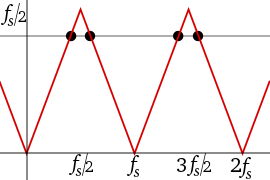
The sawtooth wave is a kind of non-sinusoidal waveform. It is so named based on its resemblance to the teeth of a plain-toothed saw with a zero rake angle. A single sawtooth, or an intermittently triggered sawtooth, is called a ramp waveform.

<span class="mw-page-title-main">Pulse-width modulation</span> Representation of a signal as a rectangular wave with varying duty cycle

Pulse-width modulation (PWM), also known as pulse-duration modulation (PDM) or pulse-length modulation (PLM), is any method of representing a signal as a rectangular wave with a varying duty cycle.

The Whittaker–Shannon interpolation formula or sinc interpolation is a method to construct a continuous-time bandlimited function from a sequence of real numbers. The formula dates back to the works of E. Borel in 1898, and E. T. Whittaker in 1915, and was cited from works of J. M. Whittaker in 1935, and in the formulation of the Nyquist–Shannon sampling theorem by Claude Shannon in 1949. It is also commonly called Shannon's interpolation formula and Whittaker's interpolation formula. E. T. Whittaker, who published it in 1915, called it the Cardinal series.

<span class="mw-page-title-main">Nyquist frequency</span> Maximum frequency of non-aliased component upon sampling

In signal processing, the Nyquist frequency, named after Harry Nyquist, is a characteristic of a sampler, which converts a continuous function or signal into a discrete sequence. For a given sampling rate, the Nyquist frequency (cycles per second) is the frequency whose cycle-length is twice the interval between samples, thus 0.5 cycle/sample. For example, audio CDs have a sampling rate of 44100 samples/second. At 0.5 cycle/sample, the corresponding Nyquist frequency is 22050 cycles/second (Hz). Conversely, the Nyquist rate for sampling a 22050 Hz signal is 44100 samples/second.

Filter design is the process of designing a signal processing filter that satisfies a set of requirements, some of which may be conflicting. The purpose is to find a realization of the filter that meets each of the requirements to a sufficient degree to make it useful.

<span class="mw-page-title-main">Sampling (signal processing)</span> Measurement of a signal at discrete time intervals

In signal processing, sampling is the reduction of a continuous-time signal to a discrete-time signal. A common example is the conversion of a sound wave to a sequence of "samples". A sample is a value of the signal at a point in time and/or space; this definition differs from the term's usage in statistics, which refers to a set of such values.

<span class="mw-page-title-main">Sine wave</span> Wave shaped like the sine function

A sine wave, sinusoidal wave, or sinusoid is a periodic wave whose waveform (shape) is the trigonometric sine function. In mechanics, as a linear motion over time, this is simple harmonic motion; as rotation, it corresponds to uniform circular motion. Sine waves occur often in physics, including wind waves, sound waves, and light waves, such as monochromatic radiation. In engineering, signal processing, and mathematics, Fourier analysis decomposes general functions into a sum of sine waves of various frequencies, relative phases, and magnitudes.

<span class="mw-page-title-main">Undersampling</span> Signal processing sample technique

In signal processing, undersampling or bandpass sampling is a technique where one samples a bandpass-filtered signal at a sample rate below its Nyquist rate, but is still able to reconstruct the signal.

The Fourier transform of a function of time, s(t), is a complex-valued function of frequency, S(f), often referred to as a frequency spectrum. Any linear time-invariant operation on s(t) produces a new spectrum of the form H(f)•S(f), which changes the relative magnitudes and/or angles (phase) of the non-zero values of S(f). Any other type of operation creates new frequency components that may be referred to as spectral leakage in the broadest sense. Sampling, for instance, produces leakage, which we call aliases of the original spectral component. For Fourier transform purposes, sampling is modeled as a product between s(t) and a Dirac comb function. The spectrum of a product is the convolution between S(f) and another function, which inevitably creates the new frequency components. But the term 'leakage' usually refers to the effect of windowing, which is the product of s(t) with a different kind of function, the window function. Window functions happen to have finite duration, but that is not necessary to create leakage. Multiplication by a time-variant function is sufficient.

<span class="mw-page-title-main">Bandlimiting</span> Limiting a signal to contain only low-frequency components

Bandlimiting refers to a process which reduces the energy of a signal to an acceptably low level outside of a desired frequency range.

An anti-aliasing filter (AAF) is a filter used before a signal sampler to restrict the bandwidth of a signal to satisfy the Nyquist–Shannon sampling theorem over the band of interest. Since the theorem states that unambiguous reconstruction of the signal from its samples is possible when the power of frequencies above the Nyquist frequency is zero, a brick wall filter is an idealized but impractical AAF. A practical AAF makes a trade off between reduced bandwidth and increased aliasing. A practical anti-aliasing filter will typically permit some aliasing to occur or attenuate or otherwise distort some in-band frequencies close to the Nyquist limit. For this reason, many practical systems sample higher than would be theoretically required by a perfect AAF in order to ensure that all frequencies of interest can be reconstructed, a practice called oversampling.

In signal processing, oversampling is the process of sampling a signal at a sampling frequency significantly higher than the Nyquist rate. Theoretically, a bandwidth-limited signal can be perfectly reconstructed if sampled at the Nyquist rate or above it. The Nyquist rate is defined as twice the bandwidth of the signal. Oversampling is capable of improving resolution and signal-to-noise ratio, and can be helpful in avoiding aliasing and phase distortion by relaxing anti-aliasing filter performance requirements.

<span class="mw-page-title-main">Delta-sigma modulation</span> Method for converting signals between digital and analog

Delta-sigma modulation is an oversampling method for encoding signals into low bit depth digital signals at a very high sample-frequency as part of the process of delta-sigma analog-to-digital converters (ADCs) and digital-to-analog converters (DACs). Delta-sigma modulation achieves high quality by utilizing a negative feedback loop during quantization to the lower bit depth that continuously corrects quantization errors and moves quantization noise to higher frequencies well above the original signal's bandwidth. Subsequent low-pass filtering for demodulation easily removes this high frequency noise and time averages to achieve high accuracy in amplitude which can be ultimately encoded as pulse-code modulation (PCM).

In a mixed-signal system, a reconstruction filter, sometimes called an anti-imaging filter, is used to construct a smooth analog signal from a digital input, as in the case of a digital to analog converter (DAC) or other sampled data output device.

In digital signal processing (DSP), a normalized frequency is a ratio of a variable frequency and a constant frequency associated with a system. Some software applications require normalized inputs and produce normalized outputs, which can be re-scaled to physical units when necessary. Mathematical derivations are usually done in normalized units, relevant to a wide range of applications.

References

  1. Mitchell, Don P.; Netravali, Arun N. (August 1988). Reconstruction filters in computer-graphics (PDF). ACM SIGGRAPH International Conference on Computer Graphics and Interactive Techniques. Vol. 22. pp. 221–228. doi:10.1145/54852.378514. ISBN   0-89791-275-6.
  2. Tessive, LLC (2010)."Time Filter Technical Explanation"
  3. Harris, Frederic J. (August 2006). Multirate Signal Processing for Communication Systems. Upper Saddle River, NJ: Prentice Hall PTR. ISBN   978-0-13-146511-4.
  4. Tukey, John W.; Hamming, R. W. (1984) [unpublished 1949]. "Measuring noise color". In Brillinger, David R. (ed.). The Collected Works of John W. Tukey. Vol. 1. Wadsworth. p. 5. ISBN   0-534-03303-2.
  5. Blackman, R. B.; J. W. Tukey (1958). "The measurement of power spectra from the point of view of communications engineering - Part I". Bell System Technical Journal . 37 (1): 216.
  6. Blackman, R. B.; J. W. Tukey (1959). The Measurement of Power Spectra from the Point of View of Communications Engineering. New York: Dover. p. vii.
  7. Stumpf, Karl (1937). Grundlagen und Methoden der Periodenforschung. Berlin: Springer. p. 45.
  8. Jenkins, G. M.; Priestley, M. B. (1957). "Discussion (Symposium on Spectral Approach to Time Series)". Journal of the Royal Statistical Society, Series B . 19 (1): 59.
  9. Finney, D. J. (1945). "The fractional replication of factorial arrangements". Annals of Eugenics. 12: 291–301. doi:10.1111/j.1469-1809.1943.tb02333.x.
  10. Tukey, John W. (1992). Cox, David R. (ed.). The Collected Works of John W. Tukey. Vol. 7. Wadsworth. ISBN   0-534-05104-9.
  11. Tukey, John W.; Hamming, R. W. (1984) [unpublished 1963]. "Mathematics 596: An introduction to the frequency analysis of time series". In Brillinger, David R. (ed.). The Collected Works of John W. Tukey. Vol. 1. Wadsworth. p. 571. ISBN   0-534-03303-2.
  12. The (New) Stanford Light Field Archive
  13. Flanagan, James L., "Beamwidth and useable bandwidth of delay-steered microphone arrays", AT&T Tech. J. , 1985, 64, pp. 983–995

Further reading