The Nyquist–Shannon sampling theorem is an essential principle for digital signal processing linking the frequency range of a signal and the sample rate required to avoid a type of distortion called aliasing. The theorem states that the sample rate must be at least twice the bandwidth of the signal to avoid aliasing distortion. In practice, it is used to select band-limiting filters to keep aliasing distortion below an acceptable amount when an analog signal is sampled or when sample rates are changed within a digital signal processing function.
A low-pass filter is a filter that passes signals with a frequency lower than a selected cutoff frequency and attenuates signals with frequencies higher than the cutoff frequency. The exact frequency response of the filter depends on the filter design. The filter is sometimes called a high-cut filter, or treble-cut filter in audio applications. A low-pass filter is the complement of a high-pass filter.

A high-pass filter (HPF) is an electronic filter that passes signals with a frequency higher than a certain cutoff frequency and attenuates signals with frequencies lower than the cutoff frequency. The amount of attenuation for each frequency depends on the filter design. A high-pass filter is usually modeled as a linear time-invariant system. It is sometimes called a low-cut filter or bass-cut filter in the context of audio engineering. High-pass filters have many uses, such as blocking DC from circuitry sensitive to non-zero average voltages or radio frequency devices. They can also be used in conjunction with a low-pass filter to produce a band-pass filter.
The Whittaker–Shannon interpolation formula or sinc interpolation is a method to construct a continuous-time bandlimited function from a sequence of real numbers. The formula dates back to the works of E. Borel in 1898, and E. T. Whittaker in 1915, and was cited from works of J. M. Whittaker in 1935, and in the formulation of the Nyquist–Shannon sampling theorem by Claude Shannon in 1949. It is also commonly called Shannon's interpolation formula and Whittaker's interpolation formula. E. T. Whittaker, who published it in 1915, called it the Cardinal series.

In signal processing, undersampling or bandpass sampling is a technique where one samples a bandpass-filtered signal at a sample rate below its Nyquist rate, but is still able to reconstruct the signal.
Chebyshev filters are analog or digital filters that have a steeper roll-off than Butterworth filters, and have either passband ripple or stopband ripple. Chebyshev filters have the property that they minimize the error between the idealized and the actual filter characteristic over the operating frequency range of the filter, but they achieve this with ripples in the passband. This type of filter is named after Pafnuty Chebyshev because its mathematical characteristics are derived from Chebyshev polynomials. Type I Chebyshev filters are usually referred to as "Chebyshev filters", while type II filters are usually called "inverse Chebyshev filters". Because of the passband ripple inherent in Chebyshev filters, filters with a smoother response in the passband but a more irregular response in the stopband are preferred for certain applications.
In mathematics, the Gibbs phenomenon is the oscillatory behavior of the Fourier series of a piecewise continuously differentiable periodic function around a jump discontinuity. The th partial Fourier series of the function produces large peaks around the jump which overshoot and undershoot the function values. As more sinusoids are used, this approximation error approaches a limit of about 9% of the jump, though the infinite Fourier series sum does eventually converge almost everywhere except points of discontinuity.
In signal processing, a finite impulse response (FIR) filter is a filter whose impulse response is of finite duration, because it settles to zero in finite time. This is in contrast to infinite impulse response (IIR) filters, which may have internal feedback and may continue to respond indefinitely.

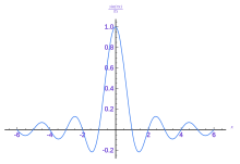
In mathematics, physics and engineering, the sinc function, denoted by sinc(x), has two forms, normalized and unnormalized.

The rectangular function is defined as

In mathematics, a Dirac comb is a periodic function with the formula
Optical resolution describes the ability of an imaging system to resolve detail, in the object that is being imaged. An imaging system may have many individual components, including one or more lenses, and/or recording and display components. Each of these contributes to the optical resolution of the system; the environment in which the imaging is done often is a further important factor.
The raised-cosine filter is a filter frequently used for pulse-shaping in digital modulation due to its ability to minimise intersymbol interference (ISI). Its name stems from the fact that the non-zero portion of the frequency spectrum of its simplest form is a cosine function, 'raised' up to sit above the (horizontal) axis.

In communications, the Nyquist ISI criterion describes the conditions which, when satisfied by a communication channel, result in no intersymbol interference or ISI. It provides a method for constructing band-limited functions to overcome the effects of intersymbol interference.

A triangular function is a function whose graph takes the shape of a triangle. Often this is an isosceles triangle of height 1 and base 2 in which case it is referred to as the triangular function. Triangular functions are useful in signal processing and communication systems engineering as representations of idealized signals, and the triangular function specifically as an integral transform kernel function from which more realistic signals can be derived, for example in kernel density estimation. It also has applications in pulse-code modulation as a pulse shape for transmitting digital signals and as a matched filter for receiving the signals. It is also used to define the triangular window sometimes called the Bartlett window.

The Hann function is named after the Austrian meteorologist Julius von Hann. It is a window function used to perform Hann smoothing. The function, with length and amplitude is given by:
The zero-order hold (ZOH) is a mathematical model of the practical signal reconstruction done by a conventional digital-to-analog converter (DAC). That is, it describes the effect of converting a discrete-time signal to a continuous-time signal by holding each sample value for one sample interval. It has several applications in electrical communication.
First-order hold (FOH) is a mathematical model of the practical reconstruction of sampled signals that could be done by a conventional digital-to-analog converter (DAC) and an analog circuit called an integrator. For FOH, the signal is reconstructed as a piecewise linear approximation to the original signal that was sampled. A mathematical model such as FOH (or, more commonly, the zero-order hold) is necessary because, in the sampling and reconstruction theorem, a sequence of Dirac impulses, xs(t), representing the discrete samples, x(nT), is low-pass filtered to recover the original signal that was sampled, x(t). However, outputting a sequence of Dirac impulses is impractical. Devices can be implemented, using a conventional DAC and some linear analog circuitry, to reconstruct the piecewise linear output for either predictive or delayed FOH.

In signal processing, particularly digital image processing, ringing artifacts are artifacts that appear as spurious signals near sharp transitions in a signal. Visually, they appear as bands or "ghosts" near edges; audibly, they appear as "echos" near transients, particularly sounds from percussion instruments; most noticeable are the pre-echos. The term "ringing" is because the output signal oscillates at a fading rate around a sharp transition in the input, similar to a bell after being struck. As with other artifacts, their minimization is a criterion in filter design.
In optics, the Fraunhofer diffraction equation is used to model the diffraction of waves when the diffraction pattern is viewed at a long distance from the diffracting object, and also when it is viewed at the focal plane of an imaging lens.