Digital image processing

This article is about mathematical processing of digital images. For artistic processing of images, see Image editing. For compression algorithms, see Image compression.

Not to be confused with Analog image processing.

Digital image processing is the use of a digital computer to process digital images through an algorithm. ^{[1] [2]} As a subcategory or field of digital signal processing, digital image processing has many advantages over analog image processing. It allows a much wider range of algorithms to be applied to the input data and can avoid problems such as the build-up of noise and distortion during processing. Since images are defined over two dimensions (perhaps more) digital image processing may be modeled in the form of multidimensional systems. The generation and development of digital image processing are mainly affected by three factors: first, the development of computers; second, the development of mathematics (especially the creation and improvement of discrete mathematics theory); third, the demand for a wide range of applications in environment, agriculture, military, industry and medical science has increased.

History

Further information: Digital image § History, and Digital imaging § History

Many of the techniques of digital image processing, or digital picture processing as it often was called, were developed in the 1960s, at Bell Laboratories, the Jet Propulsion Laboratory, Massachusetts Institute of Technology, University of Maryland, and a few other research facilities, with application to satellite imagery, wire-photo standards conversion, medical imaging, videophone, character recognition, and photograph enhancement. ^[3] The purpose of early image processing was to improve the quality of the image. It was aimed for human beings to improve the visual effect of people. In image processing, the input is a low-quality image, and the output is an image with improved quality. Common image processing include image enhancement, restoration, encoding, and compression. The first successful application was the American Jet Propulsion Laboratory (JPL). They used image processing techniques such as geometric correction, gradation transformation, noise removal, etc. on the thousands of lunar photos sent back by the Space Detector Ranger 7 in 1964, taking into account the position of the Sun and the environment of the Moon. The impact of the successful mapping of the Moon's surface map by the computer has been a success. Later, more complex image processing was performed on the nearly 100,000 photos sent back by the spacecraft, so that the topographic map, color map and panoramic mosaic of the Moon were obtained, which achieved extraordinary results and laid a solid foundation for human landing on the Moon. ^[4]

The cost of processing was fairly high, however, with the computing equipment of that era. That changed in the 1970s, when digital image processing proliferated as cheaper computers and dedicated hardware became available. This led to images being processed in real-time, for some dedicated problems such as television standards conversion. As general-purpose computers became faster, they started to take over the role of dedicated hardware for all but the most specialized and computer-intensive operations. With the fast computers and signal processors available in the 2000s, digital image processing has become the most common form of image processing, and is generally used because it is not only the most versatile method, but also the cheapest.

Image sensors

Main article: Image sensor

The basis for modern image sensors is metal–oxide–semiconductor (MOS) technology, ^[5] which originates from the invention of the MOSFET (MOS field-effect transistor) by Mohamed M. Atalla and Dawon Kahng at Bell Labs in 1959. ^[6] This led to the development of digital semiconductor image sensors, including the charge-coupled device (CCD) and later the CMOS sensor. ^[5]

The charge-coupled device was invented by Willard S. Boyle and George E. Smith at Bell Labs in 1969. ^[7] While researching MOS technology, they realized that an electric charge was the analogy of the magnetic bubble and that it could be stored on a tiny MOS capacitor. As it was fairly straightforward to fabricate a series of MOS capacitors in a row, they connected a suitable voltage to them so that the charge could be stepped along from one to the next. ^[5] The CCD is a semiconductor circuit that was later used in the first digital video cameras for television broadcasting. ^[8]

The NMOS active-pixel sensor (APS) was invented by Olympus in Japan during the mid-1980s. This was enabled by advances in MOS semiconductor device fabrication, with MOSFET scaling reaching smaller micron and then sub-micron levels. ^{[9] [10]} The NMOS APS was fabricated by Tsutomu Nakamura's team at Olympus in 1985. ^[11] The CMOS active-pixel sensor (CMOS sensor) was later developed by Eric Fossum's team at the NASA Jet Propulsion Laboratory in 1993. ^[12] By 2007, sales of CMOS sensors had surpassed CCD sensors. ^[13]

MOS image sensors are widely used in optical mouse technology. The first optical mouse, invented by Richard F. Lyon at Xerox in 1980, used a 5 µm NMOS integrated circuit sensor chip. ^{[14] [15]} Since the first commercial optical mouse, the IntelliMouse introduced in 1999, most optical mouse devices use CMOS sensors. ^{[16] [17]}

Image compression

Main article: Image compression

An important development in digital image compression technology was the discrete cosine transform (DCT), a lossy compression technique first proposed by Nasir Ahmed in 1972. ^[18] DCT compression became the basis for JPEG, which was introduced by the Joint Photographic Experts Group in 1992. ^[19] JPEG compresses images down to much smaller file sizes, and has become the most widely used image file format on the Internet. ^[20] Its highly efficient DCT compression algorithm was largely responsible for the wide proliferation of digital images and digital photos, ^[21] with several billion JPEG images produced every day as of 2015 ^[update] . ^[22]

Medical imaging techniques produce very large amounts of data, especially from CT, MRI and PET modalities. As a result, storage and communications of electronic image data are prohibitive without the use of compression. ^{[23] [24]} JPEG 2000 image compression is used by the DICOM standard for storage and transmission of medical images. The cost and feasibility of accessing large image data sets over low or various bandwidths are further addressed by use of another DICOM standard, called JPIP, to enable efficient streaming of the JPEG 2000 compressed image data. ^[25]

Digital signal processor (DSP)

Main article: Digital signal processor

Electronic signal processing was revolutionized by the wide adoption of MOS technology in the 1970s. ^[26] MOS integrated circuit technology was the basis for the first single-chip microprocessors and microcontrollers in the early 1970s, ^[27] and then the first single-chip digital signal processor (DSP) chips in the late 1970s. ^{[28] [29]} DSP chips have since been widely used in digital image processing. ^[28]

The discrete cosine transform (DCT) image compression algorithm has been widely implemented in DSP chips, with many companies developing DSP chips based on DCT technology. DCTs are widely used for encoding, decoding, video coding, audio coding, multiplexing, control signals, signaling, analog-to-digital conversion, formatting luminance and color differences, and color formats such as YUV444 and YUV411. DCTs are also used for encoding operations such as motion estimation, motion compensation, inter-frame prediction, quantization, perceptual weighting, entropy encoding, variable encoding, and motion vectors, and decoding operations such as the inverse operation between different color formats (YIQ, YUV and RGB) for display purposes. DCTs are also commonly used for high-definition television (HDTV) encoder/decoder chips. ^[30]

Medical imaging

Further information: Medical imaging

In 1972, the engineer from British company EMI Housfield invented the X-ray computed tomography device for head diagnosis, which is what is usually called CT (computer tomography). The CT nucleus method is based on the projection of the human head section and is processed by computer to reconstruct the cross-sectional image, which is called image reconstruction. In 1975, EMI successfully developed a CT device for the whole body, which obtained a clear tomographic image of various parts of the human body. In 1979, this diagnostic technique won the Nobel Prize. ^[4] Digital image processing technology for medical applications was inducted into the Space Foundation Space Technology Hall of Fame in 1994. ^[31]

As of 2010, 5 billion medical imaging studies had been conducted worldwide. ^{[32] [33]} Radiation exposure from medical imaging in 2006 made up about 50% of total ionizing radiation exposure in the United States. ^[34] Medical imaging equipment is manufactured using technology from the semiconductor industry, including CMOS integrated circuit chips, power semiconductor devices, sensors such as image sensors (particularly CMOS sensors) and biosensors, and processors such as microcontrollers, microprocessors, digital signal processors, media processors and system-on-chip devices. As of 2015 ^[update] , annual shipments of medical imaging chips amount to 46 million units and $1.1 billion. ^{[35] [36]}

Tasks

Digital image processing allows the use of much more complex algorithms, and hence, can offer both more sophisticated performance at simple tasks, and the implementation of methods which would be impossible by analogue means.

In particular, digital image processing is a concrete application of, and a practical technology based on:

• Classification
• Feature extraction
• Multi-scale signal analysis
• Pattern recognition
• Projection

Some techniques which are used in digital image processing include:

• Anisotropic diffusion
• Hidden Markov models
• Image editing
• Image restoration
• Independent component analysis
• Linear filtering
• Neural networks
• Partial differential equations
• Pixelation
• Point feature matching
• Principal components analysis
• Self-organizing maps
• Wavelets

Digital image transformations

Filtering

Digital filters are used to blur and sharpen digital images. Filtering can be performed by:

• convolution with specifically designed kernels (filter array) in the spatial domain ^[37]
• masking specific frequency regions in the frequency (Fourier) domain

The following examples show both methods: ^[38]

Filter type	Kernel or mask	Example
Original Image	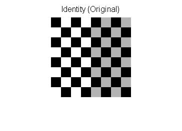${\displaystyle {\begin{bmatrix}0&0&0\\0&1&0\\0&0&0\end{bmatrix}}}$
Spatial Lowpass	${\displaystyle {\frac {1}{9}}\times {\begin{bmatrix}1&1&1\\1&1&1\\1&1&1\end{bmatrix}}}$
Spatial Highpass	${\displaystyle {\begin{bmatrix}0&-1&0\\-1&4&-1\\0&-1&0\end{bmatrix}}}$
Fourier Representation	Pseudo-code: image = checkerboard F = Fourier Transform of image Show Image: log(1+Absolute Value(F))
Fourier Lowpass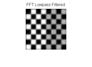
Fourier Highpass

Image padding in Fourier domain filtering

Images are typically padded before being transformed to the Fourier space, the highpass filtered images below illustrate the consequences of different padding techniques:

Zero padded	Repeated edge padded

Notice that the highpass filter shows extra edges when zero padded compared to the repeated edge padding.

Filtering code examples

MATLAB example for spatial domain highpass filtering.

img=checkerboard(20);% generate checkerboard% **************************  SPATIAL DOMAIN  ***************************klaplace=[0-10;-15-1;0-10];% Laplacian filter kernelX=conv2(img,klaplace);% convolve test img with% 3x3 Laplacian kernelfigure()imshow(X,[])% show Laplacian filteredtitle('Laplacian Edge Detection')

Affine transformations

Affine transformations enable basic image transformations including scale, rotate, translate, mirror and shear as is shown in the following examples: ^[38]

Transformation Name	Affine Matrix	Example
Identity	${\displaystyle {\begin{bmatrix}1&0&0\\0&1&0\\0&0&1\end{bmatrix}}}$
Reflection	${\displaystyle {\begin{bmatrix}-1&0&0\\0&1&0\\0&0&1\end{bmatrix}}}$
Scale	${\displaystyle {\begin{bmatrix}c_{x}=2&0&0\\0&c_{y}=1&0\\0&0&1\end{bmatrix}}}$
Rotate	${\displaystyle {\begin{bmatrix}\cos(\theta )&\sin(\theta )&0\\-\sin(\theta )&\cos(\theta )&0\\0&0&1\end{bmatrix}}}$	where θ = π/6 =30°
Shear	${\displaystyle {\begin{bmatrix}1&c_{x}=0.5&0\\c_{y}=0&1&0\\0&0&1\end{bmatrix}}}$

To apply the affine matrix to an image, the image is converted to matrix in which each entry corresponds to the pixel intensity at that location. Then each pixel's location can be represented as a vector indicating the coordinates of that pixel in the image, [x, y], where x and y are the row and column of a pixel in the image matrix. This allows the coordinate to be multiplied by an affine-transformation matrix, which gives the position that the pixel value will be copied to in the output image.

However, to allow transformations that require translation transformations, 3 dimensional homogeneous coordinates are needed. The third dimension is usually set to a non-zero constant, usually 1, so that the new coordinate is [x, y, 1]. This allows the coordinate vector to be multiplied by a 3 by 3 matrix, enabling translation shifts. So the third dimension, which is the constant 1, allows translation.

Because matrix multiplication is associative, multiple affine transformations can be combined into a single affine transformation by multiplying the matrix of each individual transformation in the order that the transformations are done. This results in a single matrix that, when applied to a point vector, gives the same result as all the individual transformations performed on the vector [x, y, 1] in sequence. Thus a sequence of affine transformation matrices can be reduced to a single affine transformation matrix.

For example, 2 dimensional coordinates only allow rotation about the origin (0, 0). But 3 dimensional homogeneous coordinates can be used to first translate any point to (0, 0), then perform the rotation, and lastly translate the origin (0, 0) back to the original point (the opposite of the first translation). These 3 affine transformations can be combined into a single matrix, thus allowing rotation around any point in the image. ^[39]

Image denoising with Morphology

Mathematical morphology is suitable for denoising images. Structuring element are important in Mathematical morphology.

The following examples are about Structuring elements. The denoise function, image as I, and structuring element as B are shown as below and table.

e.g. ${\displaystyle (I')={\begin{bmatrix}45&50&65\\40&60&55\\25&15&5\end{bmatrix}}B={\begin{bmatrix}1&2&1\\2&1&1\\1&0&3\end{bmatrix}}}$

Define Dilation(I, B)(i,j) = ${\displaystyle max\{I(i+m,j+n)+B(m,n)\}}$. Let Dilation(I,B) = D(I,B)

D(I', B)(1,1) = ${\displaystyle max(45+1,50+2,65+1,40+2,60+1,55+1,25+1,15+0,5+3)=66}$

Define Erosion(I, B)(i,j) = ${\displaystyle min\{I(i+m,j+n)-B(m,n)\}}$. Let Erosion(I,B) = E(I,B)

E(I', B)(1,1) = ${\displaystyle min(45-1,50-2,65-1,40-2,60-1,55-1,25-1,15-0,5-3)=2}$

After dilation ${\displaystyle (I')={\begin{bmatrix}45&50&65\\40&66&55\\25&15&5\end{bmatrix}}}$ After erosion ${\displaystyle (I')={\begin{bmatrix}45&50&65\\40&2&55\\25&15&5\end{bmatrix}}}$

An opening method is just simply erosion first, and then dilation while the closing method is vice versa. In reality, the D(I,B) and E(I,B) can implemented by Convolution

Structuring element	Mask	Code	Example
Original Image	None	Use Matlab to read Original image original=imread('scene.jpg');image=rgb2gray(original);[r,c,channel]=size(image);se=logical([111;111;111]);[p,q]=size(se);halfH=floor(p/2);halfW=floor(q/2);time=3;% denoising 3 times with all method	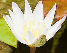Original lotus
Dilation	${\displaystyle {\begin{bmatrix}1&1&1\\1&1&1\\1&1&1\end{bmatrix}}}$	Use Matlab to dilation imwrite(image,"scene_dil.jpg")extractmax=zeros(size(image),class(image));fori=1:timedil_image=imread('scene_dil.jpg');forcol=(halfW+1):(c-halfW)forrow=(halfH+1):(r-halfH)dpointD=row-halfH;dpointU=row+halfH;dpointL=col-halfW;dpointR=col+halfW;dneighbor=dil_image(dpointD:dpointU,dpointL:dpointR);filter=dneighbor(se);extractmax(row,col)=max(filter);endendimwrite(extractmax,"scene_dil.jpg");end	Denoising picture with dilation method
Erosion	${\displaystyle {\begin{bmatrix}1&1&1\\1&1&1\\1&1&1\end{bmatrix}}}$	Use Matlab to erosion imwrite(image,'scene_ero.jpg');extractmin=zeros(size(image),class(image));fori=1:timeero_image=imread('scene_ero.jpg');forcol=(halfW+1):(c-halfW)forrow=(halfH+1):(r-halfH)pointDown=row-halfH;pointUp=row+halfH;pointLeft=col-halfW;pointRight=col+halfW;neighbor=ero_image(pointDown:pointUp,pointLeft:pointRight);filter=neighbor(se);extractmin(row,col)=min(filter);endendimwrite(extractmin,"scene_ero.jpg");end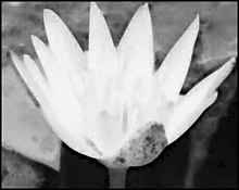
Opening	${\displaystyle {\begin{bmatrix}1&1&1\\1&1&1\\1&1&1\end{bmatrix}}}$	Use Matlab to Opening imwrite(extractmin,"scene_opening.jpg")extractopen=zeros(size(image),class(image));fori=1:timedil_image=imread('scene_opening.jpg');forcol=(halfW+1):(c-halfW)forrow=(halfH+1):(r-halfH)dpointD=row-halfH;dpointU=row+halfH;dpointL=col-halfW;dpointR=col+halfW;dneighbor=dil_image(dpointD:dpointU,dpointL:dpointR);filter=dneighbor(se);extractopen(row,col)=max(filter);endendimwrite(extractopen,"scene_opening.jpg");end
Closing	${\displaystyle {\begin{bmatrix}1&1&1\\1&1&1\\1&1&1\end{bmatrix}}}$	Use Matlab to Closing imwrite(extractmax,"scene_closing.jpg")extractclose=zeros(size(image),class(image));fori=1:timeero_image=imread('scene_closing.jpg');forcol=(halfW+1):(c-halfW)forrow=(halfH+1):(r-halfH)dpointD=row-halfH;dpointU=row+halfH;dpointL=col-halfW;dpointR=col+halfW;dneighbor=ero_image(dpointD:dpointU,dpointL:dpointR);filter=dneighbor(se);extractclose(row,col)=min(filter);endendimwrite(extractclose,"scene_closing.jpg");end	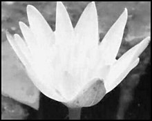Denoising picture with closing method

Applications

Further information: Digital imaging and Applications of computer vision

Digital camera images

Digital cameras generally include specialized digital image processing hardware – either dedicated chips or added circuitry on other chips – to convert the raw data from their image sensor into a color-corrected image in a standard image file format. Additional post processing techniques increase edge sharpness or color saturation to create more naturally looking images.

Film

Westworld (1973) was the first feature film to use the digital image processing to pixellate photography to simulate an android's point of view. ^[40] Image processing is also vastly used to produce the chroma key effect that replaces the background of actors with natural or artistic scenery.

Face detection

Face detection process

Face detection can be implemented with Mathematical morphology, Discrete cosine transform which is usually called DCT, and horizontal Projection (mathematics).

General method with feature-based method

The feature-based method of face detection is using skin tone, edge detection, face shape, and feature of a face (like eyes, mouth, etc.) to achieve face detection. The skin tone, face shape, and all the unique elements that only the human face have can be described as features.

Process explanation

1. Given a batch of face images, first, extract the skin tone range by sampling face images. The skin tone range is just a skin filter.
   1. Structural similarity index measure (SSIM) can be applied to compare images in terms of extracting the skin tone.
   2. Normally, HSV or RGB color spaces are suitable for the skin filter. E.g. HSV mode, the skin tone range is [0,48,50] ~ [20,255,255]
2. After filtering images with skin tone, to get the face edge, morphology and DCT are used to remove noise and fill up missing skin areas.
   1. Opening method or closing method can be used to achieve filling up missing skin.
   2. DCT is to avoid the object with tone-like skin. Since human faces always have higher texture.
   3. Sobel operator or other operators can be applied to detect face edge.
3. To position human features like eyes, using the projection and find the peak of the histogram of projection help to get the detail feature like mouth, hair, and lip.
   1. Projection is just projecting the image to see the high frequency which is usually the feature position.

Improvement of image quality method

Image quality can be influenced by camera vibration, over-exposure, gray level distribution too centralized, and noise, etc. For example, noise problem can be solved by Smoothing method while gray level distribution problem can be improved by histogram equalization.

Smoothing method

In drawing, if there is some dissatisfied color, taking some color around dissatisfied color and averaging them. This is an easy way to think of Smoothing method.

Smoothing method can be implemented with mask and Convolution. Take the small image and mask for instance as below.

image is ${\displaystyle {\begin{bmatrix}2&5&6&5\\3&1&4&6\\1&28&30&2\\7&3&2&2\end{bmatrix}}}$

mask is ${\displaystyle {\begin{bmatrix}1/9&1/9&1/9\\1/9&1/9&1/9\\1/9&1/9&1/9\end{bmatrix}}}$

After Convolution and smoothing, image is ${\displaystyle {\begin{bmatrix}2&5&6&5\\3&9&10&6\\1&9&9&2\\7&3&2&2\end{bmatrix}}}$

Oberseving image[1, 1], image[1, 2], image[2, 1], and image[2, 2].

The original image pixel is 1, 4, 28, 30. After smoothing mask, the pixel becomes 9, 10, 9, 9 respectively.

new image[1, 1] = ${\displaystyle {\tfrac {1}{9}}}$ * (image[0,0]+image[0,1]+image[0,2]+image[1,0]+image[1,1]+image[1,2]+image[2,0]+image[2,1]+image[2,2])

new image[1, 1] = floor(${\displaystyle {\tfrac {1}{9}}}$ * (2+5+6+3+1+4+1+28+30)) = 9

new image[1, 2] = floor({${\displaystyle {\tfrac {1}{9}}}$ * (5+6+5+1+4+6+28+30+2)) = 10

new image[2, 1] = floor(${\displaystyle {\tfrac {1}{9}}}$ * (3+1+4+1+28+30+7+3+2)) = 9

new image[2, 2] = floor(${\displaystyle {\tfrac {1}{9}}}$ * (1+4+6+28+30+2+3+2+2)) = 9

Gray Level Histogram method

Generally, given a gray level histogram from an image as below. Changing the histogram to uniform distribution from an image is usually what we called Histogram equalization.

Figure 1

Figure 2

In discrete time, the area of gray level histogram is ${\displaystyle \sum _{i=0}^{k}H(p_{i})}$(see figure 1) while the area of uniform distribution is ${\displaystyle \sum _{i=0}^{k}G(q_{i})}$(see figure 2). It is clear that the area will not change, so ${\displaystyle \sum _{i=0}^{k}H(p_{i})=\sum _{i=0}^{k}G(q_{i})}$.

From the uniform distribution, the probability of ${\displaystyle q_{i}}$ is ${\displaystyle {\tfrac {N^{2}}{q_{k}-q_{0}}}}$ while the ${\displaystyle 0<i<k}$

In continuous time, the equation is ${\displaystyle \displaystyle \int _{q_{0}}^{q}{\tfrac {N^{2}}{q_{k}-q_{0}}}ds=\displaystyle \int _{p_{0}}^{p}H(s)ds}$.

Moreover, based on the definition of a function, the Gray level histogram method is like finding a function ${\displaystyle f}$ that satisfies f(p)=q.

Improvement method	Issue	Before improvement	Process	After improvement
Smoothing method	noise with Matlab, salt & pepper with 0.01 parameter is added to the original image in order to create a noisy image.		read image and convert image into grayscale convolution the graysale image with the mask ${\displaystyle {\begin{bmatrix}1/9&1/9&1/9\\1/9&1/9&1/9\\1/9&1/9&1/9\end{bmatrix}}}$ denoisy image will be the result of step 2.
Histogram Equalization	Gray level distribution too centralized		Refer to the Histogram equalization

Challenges

1. Noise and Distortions : Imperfections in images due to poor lighting, limited sensors, and file compression can result in unclear images that impact accurate image conversion.
2. Variability in Image Quality: Variations in image quality and resolution, including blurry images and incomplete details, can hinder uniform processing across a database.
3. Object Detection and Recognition: Identifying and recognising objects within images, especially in complex scenarios with multiple objects and occlusions, poses a significant challenge.
4. Data Annotation and Labelling: Labelling diverse and multiple images for machine recognition is crucial for further processing accuracy, as incorrect identification can lead to unrealistic results.
5. Computational Resource Intensity : Accessing adequate computational resources for image processing can be challenging and costly, hindering progress without sufficient resources.

^[41] See also

• Digital imaging
• Computer graphics
• Computer vision
• CVIPtools
• Digitizing
• Fourier transform
• Free boundary condition
• GPGPU
• Homomorphic filtering
• Image analysis
• IEEE Intelligent Transportation Systems Society
• Least-squares spectral analysis
• Multidimensional systems
• Relaxation labelling
• Remote sensing software
• Standard test image
• Superresolution
• Total variation denoising
• Machine Vision
• Bounded variation
• Radiomics

References

1. Chakravorty, Pragnan (2018). "What is a Signal? [Lecture Notes]". IEEE Signal Processing Magazine. 35 (5): 175–177. Bibcode:2018ISPM...35e.175C. doi:10.1109/MSP.2018.2832195. S2CID   52164353.
2. Gonzalez, Rafael (2018). Digital image processing. New York, NY: Pearson. ISBN   978-0-13-335672-4. OCLC   966609831.
3. Azriel Rosenfeld, Picture Processing by Computer, New York: Academic Press, 1969
4. Gonzalez, Rafael C. (2008). Digital image processing. Woods, Richard E. (Richard Eugene), 1954– (3rd ed.). Upper Saddle River, N.J.: Prentice Hall. pp. 23–28. ISBN   978-0-13-168728-8. OCLC   137312858.
5. Williams, J. B. (2017). The Electronics Revolution: Inventing the Future. Springer. pp. 245–8. ISBN   978-3-319-49088-5.
6. "1960: Metal Oxide Semiconductor (MOS) Transistor Demonstrated". The Silicon Engine. Computer History Museum. Archived from the original on 3 October 2019. Retrieved 31 August 2019.
7. James R. Janesick (2001). Scientific charge-coupled devices. SPIE Press. pp. 3–4. ISBN   978-0-8194-3698-6.
8. Boyle, William S; Smith, George E. (1970). "Charge Coupled Semiconductor Devices". Bell Syst. Tech. J. 49 (4): 587–593. Bibcode:1970BSTJ...49..587B. doi:10.1002/j.1538-7305.1970.tb01790.x.
9. Fossum, Eric R. (12 July 1993). "Active pixel sensors: Are CCDS dinosaurs?". In Blouke, Morley M. (ed.). Charge-Coupled Devices and Solid State Optical Sensors III. Proceedings of the SPIE. Vol. 1900. pp. 2–14. Bibcode:1993SPIE.1900....2F. CiteSeerX   10.1.1.408.6558 . doi:10.1117/12.148585. S2CID   10556755.
10. Fossum, Eric R. (2007). "Active Pixel Sensors" (PDF). Eric Fossum. S2CID   18831792. Archived (PDF) from the original on 29 August 2019.
11. Matsumoto, Kazuya; et al. (1985). "A new MOS phototransistor operating in a non-destructive readout mode". Japanese Journal of Applied Physics. 24 (5A): L323. Bibcode:1985JaJAP..24L.323M. doi:10.1143/JJAP.24.L323. S2CID   108450116.
12. Fossum, Eric R.; Hondongwa, D. B. (2014). "A Review of the Pinned Photodiode for CCD and CMOS Image Sensors". IEEE Journal of the Electron Devices Society. 2 (3): 33–43. doi: 10.1109/JEDS.2014.2306412 .
13. "CMOS Image Sensor Sales Stay on Record-Breaking Pace". IC Insights. 8 May 2018. Archived from the original on 21 June 2019. Retrieved 6 October 2019.
14. Lyon, Richard F. (2014). "The Optical Mouse: Early Biomimetic Embedded Vision". Advances in Embedded Computer Vision. Springer. pp. 3–22 (3). ISBN   9783319093871.
15. Lyon, Richard F. (August 1981). "The Optical Mouse, and an Architectural Methodology for Smart Digital Sensors" (PDF). In H. T. Kung; Robert F. Sproull; Guy L. Steele (eds.). VLSI Systems and Computations. Computer Science Press. pp. 1–19. doi:10.1007/978-3-642-68402-9_1. ISBN   978-3-642-68404-3. S2CID   60722329. Archived (PDF) from the original on 26 February 2014.
16. Brain, Marshall; Carmack, Carmen (24 April 2000). "How Computer Mice Work". HowStuffWorks . Retrieved 9 October 2019.
17. Benchoff, Brian (17 April 2016). "Building the First Digital Camera". Hackaday . Retrieved 30 April 2016. the Cyclops was the first digital camera
18. Ahmed, Nasir (January 1991). "How I Came Up With the Discrete Cosine Transform". Digital Signal Processing . 1 (1): 4–5. Bibcode:1991DSP.....1....4A. doi:10.1016/1051-2004(91)90086-Z. Archived from the original on 10 June 2016. Retrieved 10 October 2019.
19. "T.81 – Digital compression and coding of continuous-tone still images – requirements and guidelines" (PDF). CCITT. September 1992. Archived (PDF) from the original on 17 July 2019. Retrieved 12 July 2019.
20. Svetlik, Joe (31 May 2018). "The JPEG image format explained". BT Group. Archived from the original on 5 August 2019. Retrieved 5 August 2019.
21. Caplan, Paul (24 September 2013). "What Is a JPEG? The Invisible Object You See Every Day" . The Atlantic . Archived from the original on 9 October 2019. Retrieved 13 September 2019.
22. Baraniuk, Chris (15 October 2015). "JPeg lockdown: Restriction options sought by committee". BBC News. Archived from the original on 9 October 2019. Retrieved 13 September 2019.
23. Nagornov, Nikolay N.; Lyakhov, Pavel A.; Valueva, Maria V.; Bergerman, Maxim V. (2022). "RNS-Based FPGA Accelerators for High-Quality 3D Medical Image Wavelet Processing Using Scaled Filter Coefficients". IEEE Access. 10: 19215–19231. Bibcode:2022IEEEA..1019215N. doi: 10.1109/ACCESS.2022.3151361 . ISSN   2169-3536. S2CID   246895876 . Medical imaging systems produce increasingly accurate images with improved quality using higher spatial resolutions and color bit-depth. Such improvements increase the amount of information that needs to be stored, processed, and transmitted.
24. Dhouib, D.; Naït-Ali, A.; Olivier, C.; Naceur, M.S. (June 2021). "ROI-Based Compression Strategy of 3D MRI Brain Datasets for Wireless Communications". IRBM. 42 (3): 146–153. doi:10.1016/j.irbm.2020.05.001. S2CID   219437400. Because of the large amount of medical imaging data, the transmission process becomes complicated in telemedicine applications. Thus, in order to adapt the data bit streams to the constraints related to the limitation of the bandwidths a reduction of the size of the data by compression of the images is essential.
25. Xin, Gangtao; Fan, Pingyi (11 June 2021). "A lossless compression method for multi-component medical images based on big data mining". Scientific Reports. 11 (1): 12372. doi: 10.1038/s41598-021-91920-x . ISSN   2045-2322. PMC   8196061 . PMID   34117350.
26. Grant, Duncan Andrew; Gowar, John (1989). Power MOSFETS: theory and applications. Wiley. p. 1. ISBN   978-0-471-82867-9. The metal–oxide–semiconductor field-effect transistor (MOSFET) is the most commonly used active device in the very large-scale integration of digital integrated circuits (VLSI). During the 1970s these components revolutionized electronic signal processing, control systems and computers.
27. Shirriff, Ken (30 August 2016). "The Surprising Story of the First Microprocessors". IEEE Spectrum . 53 (9). Institute of Electrical and Electronics Engineers: 48–54. doi:10.1109/MSPEC.2016.7551353. S2CID   32003640. Archived from the original on 13 October 2019. Retrieved 13 October 2019.
28. "1979: Single Chip Digital Signal Processor Introduced". The Silicon Engine. Computer History Museum. Archived from the original on 3 October 2019. Retrieved 14 October 2019.
29. Taranovich, Steve (27 August 2012). "30 years of DSP: From a child's toy to 4G and beyond". EDN . Archived from the original on 14 October 2019. Retrieved 14 October 2019.
30. Stanković, Radomir S.; Astola, Jaakko T. (2012). "Reminiscences of the Early Work in DCT: Interview with K.R. Rao" (PDF). Reprints from the Early Days of Information Sciences. 60. Archived (PDF) from the original on 13 October 2019. Retrieved 13 October 2019.
31. "Space Technology Hall of Fame:Inducted Technologies/1994". Space Foundation. 1994. Archived from the original on 4 July 2011. Retrieved 7 January 2010.
32. Roobottom CA, Mitchell G, Morgan-Hughes G (November 2010). "Radiation-reduction strategies in cardiac computed tomographic angiography". Clinical Radiology. 65 (11): 859–67. doi: 10.1016/j.crad.2010.04.021 . PMID   20933639.
33. Scialpi M, Reginelli A, D'Andrea A, Gravante S, Falcone G, Baccari P, Manganaro L, Palumbo B, Cappabianca S (April 2016). "Pancreatic tumors imaging: An update" (PDF). International Journal of Surgery. 28 (Suppl 1): S142-55. doi: 10.1016/j.ijsu.2015.12.053 . hdl:11573/908479. PMID   26777740. Archived (PDF) from the original on 24 August 2019.
34. Rahbar H, Partridge SC (February 2016). "Multiparametric MR Imaging of Breast Cancer". Magnetic Resonance Imaging Clinics of North America. 24 (1): 223–238. doi:10.1016/j.mric.2015.08.012. PMC   4672390 . PMID   26613883.
35. "Medical Imaging Chip Global Unit Volume To Soar Over the Next Five Years". Silicon Semiconductor. 8 September 2016. Retrieved 25 October 2019.
36. Banerjee R, Pavlides M, Tunnicliffe EM, Piechnik SK, Sarania N, Philips R, Collier JD, Booth JC, Schneider JE, Wang LM, Delaney DW, Fleming KA, Robson MD, Barnes E, Neubauer S (January 2014). "Multiparametric magnetic resonance for the non-invasive diagnosis of liver disease". Journal of Hepatology. 60 (1): 69–77. doi:10.1016/j.jhep.2013.09.002. PMC   3865797 . PMID   24036007.
37. Zhang, M. Z.; Livingston, A. R.; Asari, V. K. (2008). "A High Performance Architecture for Implementation of 2-D Convolution with Quadrant Symmetric Kernels". International Journal of Computers and Applications. 30 (4): 298–308. doi:10.1080/1206212x.2008.11441909. S2CID   57289814.
38. Gonzalez, Rafael (2008). Digital Image Processing, 3rd. Pearson Hall. ISBN   978-0-13-168728-8.
39. House, Keyser (6 December 2016). Affine Transformations (PDF). Foundations of Physically Based Modeling & Animation. A K Peters/CRC Press. ISBN   978-1-4822-3460-2. Archived (PDF) from the original on 30 August 2017. Retrieved 26 March 2019.{{cite book}}: |website= ignored (help)
40. A Brief, Early History of Computer Graphics in Film Archived 17 July 2012 at the Wayback Machine , Larry Yaeger, 16 August 2002 (last update), retrieved 24 March 2010
41. Barni, Mauro (September 2005). "Image Processing for the Analysis and Conservation of Paintings: Opportunities and Challenges". IEEE Signal Processing Magazine. 22 (5): 141. Bibcode:2005ISPM...22..141B. doi:10.1109/MSP.2005.1511835.

Further reading

• Solomon, C.J.; Breckon, T.P. (2010). Fundamentals of Digital Image Processing: A Practical Approach with Examples in Matlab. Wiley-Blackwell. doi:10.1002/9780470689776. ISBN   978-0-470-84473-1.
• Wilhelm Burger; Mark J. Burge (2007). Digital Image Processing: An Algorithmic Approach Using Java. Springer. ISBN   978-1-84628-379-6.
• R. Fisher; K Dawson-Howe; A. Fitzgibbon; C. Robertson; E. Trucco (2005). Dictionary of Computer Vision and Image Processing. John Wiley. ISBN   978-0-470-01526-1.
• Rafael C. Gonzalez; Richard E. Woods; Steven L. Eddins (2004). Digital Image Processing using MATLAB. Pearson Education. ISBN   978-81-7758-898-9.
• Tim Morris (2004). Computer Vision and Image Processing. Palgrave Macmillan. ISBN   978-0-333-99451-1.
• Vipin Tyagi (2018). Understanding Digital Image Processing. Taylor and Francis CRC Press. ISBN   978-11-3856-6842.
• Milan Sonka; Vaclav Hlavac; Roger Boyle (1999). Image Processing, Analysis, and Machine Vision. PWS Publishing. ISBN   978-0-534-95393-5.
• Gonzalez, Rafael C.; Woods, Richard E. (2008). Digital image processing. Upper Saddle River, N.J.: Prentice Hall. ISBN   978-0-13-168728-8. OCLC   137312858.
• Kovalevsky, Vladimir (2019). Modern algorithms for image processing: computer imagery by example using C#. [New York, New York]. ISBN   978-1-4842-4237-7. OCLC   1080084533.

External links

• Lectures on Image Processing, by Alan Peters. Vanderbilt University. Updated 7 January 2016.
• Processing digital images with computer algorithms