Gaussian adaptation (GA), also called normal or natural adaptation (NA) is an evolutionary algorithm designed for the maximization of manufacturing yield due to statistical deviation of component values of signal processing systems. In short, GA is a stochastic adaptive process where a number of samples of an n-dimensional vector x[xT = (x1, x2, ..., xn)] are taken from a multivariate Gaussian distribution, N(m,M), having mean m and moment matrixM. The samples are tested for fail or pass. The first- and second-order moments of the Gaussian restricted to the pass samples are m* andM*.
The outcome of x as a pass sample is determined by a function s(x), 0<s(x)<q≤1, such that s(x) is the probability that x will be selected as a pass sample. The average probability of finding pass samples (yield) is
Then the theorem of GA states:
For any s(x) and for any value of P<q, there always exist a Gaussian p. d. f. [ probability density function ] that is adapted for maximum dispersion. The necessary conditions for a local optimum are m=m* and M proportional to M*. The dual problem is also solved: P is maximized while keeping the dispersion constant (Kjellström, 1991).
Proofs of the theorem may be found in the papers by Kjellström, 1970, and Kjellström & Taxén, 1981.
Since dispersion is defined as the exponential of entropy/disorder/average information it immediately follows that the theorem is valid also for those concepts. Altogether, this means that Gaussian adaptation may carry out a simultaneous maximisation of yield and average information (without any need for the yield or the average information to be defined as criterion functions).
The theorem is valid for all regions of acceptability and all Gaussian distributions. It may be used by cyclic repetition of random variation and selection (like the natural evolution). In every cycle a sufficiently large number of Gaussian distributed points are sampled and tested for membership in the region of acceptability. The centre of gravity of the Gaussian, m, is then moved to the centre of gravity of the approved (selected) points, m*. Thus, the process converges to a state of equilibrium fulfilling the theorem. A solution is always approximate because the centre of gravity is always determined for a limited number of points.
It was used for the first time in 1969 as a pure optimization algorithm making the regions of acceptability smaller and smaller (in analogy to simulated annealing, Kirkpatrick 1983). Since 1970 it has been used for both ordinary optimization and yield maximization.
Natural evolution and Gaussian adaptation
It has also been compared to the natural evolution of populations of living organisms. In this case s(x) is the probability that the individual having an array x of phenotypes will survive by giving offspring to the next generation; a definition of individual fitness given by Hartl 1981. The yield, P, is replaced by the mean fitness determined as a mean over the set of individuals in a large population.
Phenotypes are often Gaussian distributed in a large population and a necessary condition for the natural evolution to be able to fulfill the theorem of Gaussian adaptation, with respect to all Gaussian quantitative characters, is that it may push the centre of gravity of the Gaussian to the centre of gravity of the selected individuals. This may be accomplished by the Hardy–Weinberg law. This is possible because the theorem of Gaussian adaptation is valid for any region of acceptability independent of the structure (Kjellström, 1996).
In this case the rules of genetic variation such as crossover, inversion, transposition etcetera may be seen as random number generators for the phenotypes. So, in this sense Gaussian adaptation may be seen as a genetic algorithm.
How to climb a mountain
Mean fitness may be calculated provided that the distribution of parameters and the structure of the landscape is known. The real landscape is not known, but figure below shows a fictitious profile (blue) of a landscape along a line (x) in a room spanned by such parameters. The red curve is the mean based on the red bell curve at the bottom of figure. It is obtained by letting the bell curve slide along the x-axis, calculating the mean at every location. As can be seen, small peaks and pits are smoothed out. Thus, if evolution is started at A with a relatively small variance (the red bell curve), then climbing will take place on the red curve. The process may get stuck for millions of years at B or C, as long as the hollows to the right of these points remain, and the mutation rate is too small.
If the mutation rate is sufficiently high, the disorder or variance may increase and the parameter(s) may become distributed like the green bell curve. Then the climbing will take place on the green curve, which is even more smoothed out. Because the hollows to the right of B and C have now disappeared, the process may continue up to the peaks at D. But of course the landscape puts a limit on the disorder or variability. Besides — dependent on the landscape — the process may become very jerky, and if the ratio between the time spent by the process at a local peak and the time of transition to the next peak is very high, it may as well look like a punctuated equilibrium as suggested by Gould (see Ridley).
Computer simulation of Gaussian adaptation
Thus far the theory only considers mean values of continuous distributions corresponding to an infinite number of individuals. In reality however, the number of individuals is always limited, which gives rise to an uncertainty in the estimation of m and M (the moment matrix of the Gaussian). And this may also affect the efficiency of the process. Unfortunately very little is known about this, at least theoretically.
The implementation of normal adaptation on a computer is a fairly simple task. The adaptation of m may be done by one sample (individual) at a time, for example
m(i + 1) = (1 – a) m(i) + ax
where x is a pass sample, and a < 1 a suitable constant so that the inverse of a represents the number of individuals in the population.
M may in principle be updated after every step y leading to a feasible point
x = m + y according to:
M(i + 1) = (1 – 2b) M(i) + 2byyT,
where yT is the transpose of y and b << 1 is another suitable constant. In order to guarantee a suitable increase of average information, y should be normally distributed with moment matrix μ2M, where the scalar μ > 1 is used to increase average information (information entropy, disorder, diversity) at a suitable rate. But M will never be used in the calculations. Instead we use the matrix W defined by WWT = M.
Thus, we have y = Wg, where g is normally distributed with the moment matrix μU, and U is the unit matrix. W and WT may be updated by the formulas
W = (1 – b)W + bygT and WT = (1 – b)WT + bgyT
because multiplication gives
M = (1 – 2b)M + 2byyT,
where terms including b2 have been neglected. Thus, M will be indirectly adapted with good approximation. In practice it will suffice to update W only
W(i + 1) = (1 – b)W(i) + bygT.
This is the formula used in a simple 2-dimensional model of a brain satisfying the Hebbian rule of associative learning; see the next section (Kjellström, 1996 and 1999).
The figure below illustrates the effect of increased average information in a Gaussian p.d.f. used to climb a mountain Crest (the two lines represent the contour line). Both the red and green cluster have equal mean fitness, about 65%, but the green cluster has a much higher average information making the green process much more efficient. The effect of this adaptation is not very salient in a 2-dimensional case, but in a high-dimensional case, the efficiency of the search process may be increased by many orders of magnitude.
The evolution in the brain
In the brain the evolution of DNA-messages is supposed to be replaced by an evolution of signal patterns and the phenotypic landscape is replaced by a mental landscape, the complexity of which will hardly be second to the former. The metaphor with the mental landscape is based on the assumption that certain signal patterns give rise to a better well-being or performance. For instance, the control of a group of muscles leads to a better pronunciation of a word or performance of a piece of music.
In this simple model it is assumed that the brain consists of interconnected components that may add, multiply and delay signal values.
A nerve cell kernel may add signal values,
a synapse may multiply with a constant and
An axon may delay values.
This is a basis of the theory of digital filters and neural networks consisting of components that may add, multiply and delay signalvalues and also of many brain models, Levine 1991.
In the figure below the brain stem is supposed to deliver Gaussian distributed signal patterns. This may be possible since certain neurons fire at random (Kandel et al.). The stem also constitutes a disordered structure surrounded by more ordered shells (Bergström, 1969), and according to the central limit theorem the sum of signals from many neurons may be Gaussian distributed. The triangular boxes represent synapses and the boxes with the + sign are cell kernels.
In the cortex signals are supposed to be tested for feasibility. When a signal is accepted the contact areas in the synapses are updated according to the formulas below in agreement with the Hebbian theory. The figure shows a 2-dimensional computer simulation of Gaussian adaptation according to the last formula in the preceding section.
As can be seen this is very much like a small brain ruled by the theory of Hebbian learning (Kjellström, 1996, 1999 and 2002).
Gaussian adaptation and free will
Gaussian adaptation as an evolutionary model of the brain obeying the Hebbian theory of associative learning offers an alternative view of free will due to the ability of the process to maximize the mean fitness of signal patterns in the brain by climbing a mental landscape in analogy with phenotypic evolution.
Such a random process gives us much freedom of choice, but hardly any will. An illusion of will may, however, emanate from the ability of the process to maximize mean fitness, making the process goal seeking. I. e., it prefers higher peaks in the landscape prior to lower, or better alternatives prior to worse. In this way an illusive will may appear. A similar view has been given by Zohar 1990. See also Kjellström 1999.
A theorem of efficiency for random search
The efficiency of Gaussian adaptation relies on the theory of information due to Claude E. Shannon (see information content). When an event occurs with probability P, then the information −log(P) may be achieved. For instance, if the mean fitness is P, the information gained for each individual selected for survival will be −log(P) – on the average - and the work/time needed to get the information is proportional to 1/P. Thus, if efficiency, E, is defined as information divided by the work/time needed to get it we have:
E = −P log(P).
This function attains its maximum when P = 1/e = 0.37. The same result has been obtained by Gaines with a different method.
E = 0 if P = 0, for a process with infinite mutation rate, and if P = 1, for a process with mutation rate = 0 (provided that the process is alive). This measure of efficiency is valid for a large class of random search processes provided that certain conditions are at hand.
1 The search should be statistically independent and equally efficient in different parameter directions. This condition may be approximately fulfilled when the moment matrix of the Gaussian has been adapted for maximum average information to some region of acceptability, because linear transformations of the whole process do not affect efficiency.
2 All individuals have equal cost and the derivative at P = 1 is <0.
Then, the following theorem may be proved:
All measures of efficiency, that satisfy the conditions above, are asymptotically proportional to –P log(P/q) when the number of dimensions increases, and are maximized by P = q exp(-1) (Kjellström, 1996 and 1999).
The figure above shows a possible efficiency function for a random search process such as Gaussian adaptation. To the left the process is most chaotic when P = 0, while there is perfect order to the right where P = 1.
In an example by Rechenberg, 1971, 1973, a random walk is pushed thru a corridor maximizing the parameter x1. In this case the region of acceptability is defined as a (n−1)-dimensional interval in the parameters x2, x3, ..., xn, but a x1-value below the last accepted will never be accepted. Since P can never exceed 0.5 in this case, the maximum speed towards higher x1-values is reached for P = 0.5/e = 0.18, in agreement with the findings of Rechenberg.
A point of view that also may be of interest in this context is that no definition of information (other than that sampled points inside some region of acceptability gives information about the extension of the region) is needed for the proof of the theorem. Then, because, the formula may be interpreted as information divided by the work needed to get the information, this is also an indication that −log(P) is a good candidate for being a measure of information.
The Stauffer and Grimson algorithm
Gaussian adaptation has also been used for other purposes as for instance shadow removal by "The Stauffer-Grimson algorithm" which is equivalent to Gaussian adaptation as used in the section "Computer simulation of Gaussian adaptation" above. In both cases the maximum likelihood method is used for estimation of mean values by adaptation at one sample at a time.
But there are differences. In the Stauffer-Grimson case the information is not used for the control of a random number generator for centering, maximization of mean fitness, average information or manufacturing yield. The adaptation of the moment matrix also differs very much as compared to "the evolution in the brain" above.
In computer science and operations research, a genetic algorithm (GA) is a metaheuristic inspired by the process of natural selection that belongs to the larger class of evolutionary algorithms (EA). Genetic algorithms are commonly used to generate high-quality solutions to optimization and search problems by relying on biologically inspired operators such as mutation, crossover and selection. Some examples of GA applications include optimizing decision trees for better performance, solving sudoku puzzles, hyperparameter optimization, causal inference, etc.
In signal processing, white noise is a random signal having equal intensity at different frequencies, giving it a constant power spectral density. The term is used, with this or similar meanings, in many scientific and technical disciplines, including physics, acoustical engineering, telecommunications, and statistical forecasting. White noise refers to a statistical model for signals and signal sources, rather than to any specific signal. White noise draws its name from white light, although light that appears white generally does not have a flat power spectral density over the visible band.
In statistics, maximum likelihood estimation (MLE) is a method of estimating the parameters of an assumed probability distribution, given some observed data. This is achieved by maximizing a likelihood function so that, under the assumed statistical model, the observed data is most probable. The point in the parameter space that maximizes the likelihood function is called the maximum likelihood estimate. The logic of maximum likelihood is both intuitive and flexible, and as such the method has become a dominant means of statistical inference.
In computational intelligence (CI), an evolutionary algorithm (EA) is a subset of evolutionary computation, a generic population-based metaheuristic optimization algorithm. An EA uses mechanisms inspired by biological evolution, such as reproduction, mutation, recombination, and selection. Candidate solutions to the optimization problem play the role of individuals in a population, and the fitness function determines the quality of the solutions. Evolution of the population then takes place after the repeated application of the above operators.
In probability theory and statistics, a Gaussian process is a stochastic process, such that every finite collection of those random variables has a multivariate normal distribution, i.e. every finite linear combination of them is normally distributed. The distribution of a Gaussian process is the joint distribution of all those random variables, and as such, it is a distribution over functions with a continuous domain, e.g. time or space.
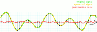
Quantization, in mathematics and digital signal processing, is the process of mapping input values from a large set to output values in a (countable) smaller set, often with a finite number of elements. Rounding and truncation are typical examples of quantization processes. Quantization is involved to some degree in nearly all digital signal processing, as the process of representing a signal in digital form ordinarily involves rounding. Quantization also forms the core of essentially all lossy compression algorithms.
In information theory and statistics, negentropy is used as a measure of distance to normality. The concept and phrase "negative entropy" was introduced by Erwin Schrödinger in his 1944 popular-science book What is Life? Later, French physicist Léon Brillouin shortened the phrase to néguentropie (negentropy). In 1974, Albert Szent-Györgyi proposed replacing the term negentropy with syntropy. That term may have originated in the 1940s with the Italian mathematician Luigi Fantappiè, who tried to construct a unified theory of biology and physics. Buckminster Fuller tried to popularize this usage, but negentropy remains common.
Fisher's fundamental theorem of natural selection is an idea about genetic variance in population genetics developed by the statistician and evolutionary biologist Ronald Fisher. The proper way of applying the abstract mathematics of the theorem to actual biology has been a matter of some debate.
In signal processing, independent component analysis (ICA) is a computational method for separating a multivariate signal into additive subcomponents. This is done by assuming that at most one subcomponent is Gaussian and that the subcomponents are statistically independent from each other. ICA is a special case of blind source separation. A common example application is the "cocktail party problem" of listening in on one person's speech in a noisy room.
A sensor array is a group of sensors, usually deployed in a certain geometry pattern, used for collecting and processing electromagnetic or acoustic signals. The advantage of using a sensor array over using a single sensor lies in the fact that an array adds new dimensions to the observation, helping to estimate more parameters and improve the estimation performance. For example an array of radio antenna elements used for beamforming can increase antenna gain in the direction of the signal while decreasing the gain in other directions, i.e., increasing signal-to-noise ratio (SNR) by amplifying the signal coherently. Another example of sensor array application is to estimate the direction of arrival of impinging electromagnetic waves. The related processing method is called array signal processing. A third examples includes chemical sensor arrays, which utilize multiple chemical sensors for fingerprint detection in complex mixtures or sensing environments. Application examples of array signal processing include radar/sonar, wireless communications, seismology, machine condition monitoring, astronomical observations fault diagnosis, etc.
Covariance matrix adaptation evolution strategy (CMA-ES) is a particular kind of strategy for numerical optimization. Evolution strategies (ES) are stochastic, derivative-free methods for numerical optimization of non-linear or non-convex continuous optimization problems. They belong to the class of evolutionary algorithms and evolutionary computation. An evolutionary algorithm is broadly based on the principle of biological evolution, namely the repeated interplay of variation and selection: in each generation (iteration) new individuals are generated by variation, usually in a stochastic way, of the current parental individuals. Then, some individuals are selected to become the parents in the next generation based on their fitness or objective function value . Like this, over the generation sequence, individuals with better and better -values are generated.
In various science/engineering applications, such as independent component analysis, image analysis, genetic analysis, speech recognition, manifold learning, and time delay estimation it is useful to estimate the differential entropy of a system or process, given some observations.
In probability theory and statistics, a collection of random variables is independent and identically distributed if each random variable has the same probability distribution as the others and all are mutually independent. This property is usually abbreviated as i.i.d., iid, or IID. IID was first defined in statistics and finds application in different fields such as data mining and signal processing.
Natural evolution strategies (NES) are a family of numerical optimization algorithms for black box problems. Similar in spirit to evolution strategies, they iteratively update the (continuous) parameters of a search distribution by following the natural gradient towards higher expected fitness.
Joint Approximation Diagonalization of Eigen-matrices (JADE) is an algorithm for independent component analysis that separates observed mixed signals into latent source signals by exploiting fourth order moments. The fourth order moments are a measure of non-Gaussianity, which is used as a proxy for defining independence between the source signals. The motivation for this measure is that Gaussian distributions possess zero excess kurtosis, and with non-Gaussianity being a canonical assumption of ICA, JADE seeks an orthogonal rotation of the observed mixed vectors to estimate source vectors which possess high values of excess kurtosis.
In statistics, Whittle likelihood is an approximation to the likelihood function of a stationary Gaussian time series. It is named after the mathematician and statistician Peter Whittle, who introduced it in his PhD thesis in 1951. It is commonly used in time series analysis and signal processing for parameter estimation and signal detection.
The following outline is provided as an overview of and topical guide to machine learning. Machine learning is a subfield of soft computing within computer science that evolved from the study of pattern recognition and computational learning theory in artificial intelligence. In 1959, Arthur Samuel defined machine learning as a "field of study that gives computers the ability to learn without being explicitly programmed". Machine learning explores the study and construction of algorithms that can learn from and make predictions on data. Such algorithms operate by building a model from an example training set of input observations in order to make data-driven predictions or decisions expressed as outputs, rather than following strictly static program instructions.
Probabilistic numerics is an active field of study at the intersection of applied mathematics, statistics, and machine learning centering on the concept of uncertainty in computation. In probabilistic numerics, tasks in numerical analysis such as finding numerical solutions for integration, linear algebra, optimization and simulation and differential equations are seen as problems of statistical, probabilistic, or Bayesian inference.
References
Bergström, R. M. An Entropy Model of the Developing Brain. Developmental Psychobiology, 2(3): 139–152, 1969.
Brooks, D. R. & Wiley, E. O. Evolution as Entropy, Towards a unified theory of Biology. The University of Chicago Press, 1986.
Brooks, D. R. Evolution in the Information Age: Rediscovering the Nature of the Organism. Semiosis, Evolution, Energy, Development, Volume 1, Number 1, March 2001
Gaines, Brian R. Knowledge Management in Societies of Intelligent Adaptive Agents. Journal of intelligent Information systems 9, 277–298 (1997).
Hartl, D. L. A Primer of Population Genetics. Sinauer, Sunderland, Massachusetts, 1981.
Hamilton, WD. 1963. The evolution of altruistic behavior. American Naturalist 97:354–356
Kandel, E. R., Schwartz, J. H., Jessel, T. M. Essentials of Neural Science and Behavior. Prentice Hall International, London, 1995.
S. Kirkpatrick and C. D. Gelatt and M. P. Vecchi, Optimization by Simulated Annealing, Science, Vol 220, Number 4598, pages 671–680, 1983.
Kjellström, G. Network Optimization by Random Variation of component values. Ericsson Technics, vol. 25, no. 3, pp.133–151, 1969.
Kjellström, G. Optimization of electrical Networks with respect to Tolerance Costs. Ericsson Technics, no. 3, pp.157–175, 1970.
Kjellström, G. & Taxén, L. Stochastic Optimization in System Design. IEEE Trans. on Circ. and Syst., vol. CAS-28, no. 7, July 1981.
Kjellström, G., Taxén, L. and Lindberg, P. O. Discrete Optimization of Digital Filters Using Gaussian Adaptation and Quadratic Function Minimization. IEEE Trans. on Circ. and Syst., vol. CAS-34, no 10, October 1987.
Kjellström, G. On the Efficiency of Gaussian Adaptation. Journal of Optimization Theory and Applications, vol. 71, no. 3, December 1991.
Kjellström, G. & Taxén, L. Gaussian Adaptation, an evolution-based efficient global optimizer; Computational and Applied Mathematics, In, C. Brezinski & U. Kulish (Editors), Elsevier Science Publishers B. V., pp 267–276, 1992.
Kjellström, G. Evolution as a statistical optimization algorithm. Evolutionary Theory 11:105–117 (January, 1996).
Kjellström, G. The evolution in the brain. Applied Mathematics and Computation, 98(2–3):293–300, February, 1999.
Kjellström, G. Evolution in a nutshell and some consequences concerning valuations. EVOLVE, ISBN91-972936-1-X, Stockholm, 2002.
Levine, D. S. Introduction to Neural & Cognitive Modeling. Laurence Erlbaum Associates, Inc., Publishers, 1991.
MacLean, P. D. A Triune Concept of the Brain and Behavior. Toronto, Univ. Toronto Press, 1973.
Maynard Smith, J. 1964. Group Selection and Kin Selection, Nature 201:1145–1147.
Maynard Smith, J. Evolutionary Genetics. Oxford University Press, 1998.
Mayr, E. What Evolution is. Basic Books, New York, 2001.
Müller, Christian L. and Sbalzarini Ivo F. Gaussian Adaptation revisited - an entropic view on Covariance Matrix Adaptation. Institute of Theoretical Computer Science and Swiss Institute of Bioinformatics, ETH Zurich, CH-8092 Zurich, Switzerland.
Pinel, J. F. and Singhal, K. Statistical Design Centering and Tolerancing Using Parametric Sampling. IEEE Transactions on Circuits and Systems, Vol. Das-28, No. 7, July 1981.
Rechenberg, I. (1971): Evolutionsstrategie — Optimierung technischer Systeme nach Prinzipien der biologischen Evolution (PhD thesis). Reprinted by Fromman-Holzboog (1973).
Ridley, M. Evolution. Blackwell Science, 1996.
Stauffer, C. & Grimson, W.E.L. Learning Patterns of Activity Using Real-Time Tracking, IEEE Trans. on PAMI, 22(8), 2000.
Stehr, G. On the Performance Space Exploration of Analog Integrated Circuits. Technischen Universität Munchen, Dissertation 2005.
Taxén, L. A Framework for the Coordination of Complex Systems’ Development. Institute of Technology, Linköping University, Dissertation, 2003.
Zohar, D. The quantum self: a revolutionary view of human nature and consciousness rooted in the new physics. London, Bloomsbury, 1990.
This page is based on this Wikipedia article Text is available under the CC BY-SA 4.0 license; additional terms may apply. Images, videos and audio are available under their respective licenses.