In mathematics, an inequality is a relation which makes a non-equal comparison between two numbers or other mathematical expressions.[1] It is used most often to compare two numbers on the number line by their size. The main types of inequality are less than and greater than.
There are several different notations used to represent different kinds of inequalities:
The notation a < b means that a is less thanb.
The notation a > b means that a is greater thanb.
In either case, a is not equal to b. These relations are known as strict inequalities,[1] meaning that a is strictly less than or strictly greater than b. Equality is excluded.
In contrast to strict inequalities, there are two types of inequality relations that are not strict:
The notation a ≤ b or a ⩽ b means that a is less than or equal tob (or, equivalently, at most b, or not greater than b).
The notation a ≥ b or a ⩾ b means that a is greater than or equal tob (or, equivalently, at least b, or not less than b).
The relation not greater than can also be represented by the symbol for "greater than" bisected by a slash, "not". The same is true for not less than,
The notation a ≠ b means that a is not equal to b; this inequation sometimes is considered a form of strict inequality.[2] It does not say that one is greater than the other; it does not even require a and b to be member of an ordered set.
In engineering sciences, less formal use of the notation is to state that one quantity is "much greater" than another,[3] normally by several orders of magnitude.
The notation a ≪ b means that a is much less thanb.[4]
The notation a ≫ b means that a is much greater thanb.[5]
This implies that the lesser value can be neglected with little effect on the accuracy of an approximation (such as the case of ultrarelativistic limit in physics).
In all of the cases above, any two symbols mirroring each other are symmetrical; a < b and b > a are equivalent, etc.
Properties on the number line
Inequalities are governed by the following properties. All of these properties also hold if all of the non-strict inequalities (≤ and ≥) are replaced by their corresponding strict inequalities (< and >) and — in the case of applying a function — monotonic functions are limited to strictlymonotonic functions.
Converse
The relations ≤ and ≥ are each other's converse, meaning that for any real numbersa and b:
a ≤ b and b ≥ a are equivalent.
Transitivity
The transitive property of inequality states that for any real numbersa, b, c:[6]
If a ≤ b and b ≤ c, then a ≤ c.
If either of the premises is a strict inequality, then the conclusion is a strict inequality:
In other words, the inequality relation is preserved under addition (or subtraction) and the real numbers are an ordered group under addition.
Multiplication and division
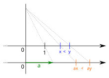
If x < y and a > 0, then ax < ay.If x < y and a < 0, then ax > ay.
The properties that deal with multiplication and division state that for any real numbers, a, b and non-zero c:
If a ≤ b and c > 0, then ac ≤ bc and a/c ≤ b/c.
If a ≤ b and c < 0, then ac ≥ bc and a/c ≥ b/c.
In other words, the inequality relation is preserved under multiplication and division with positive constant, but is reversed when a negative constant is involved. More generally, this applies for an ordered field. For more information, see § Ordered fields.
Additive inverse
The property for the additive inverse states that for any real numbers a and b:
If a ≤ b, then −a ≥ −b.
Multiplicative inverse
If both numbers are positive, then the inequality relation between the multiplicative inverses is opposite of that between the original numbers. More specifically, for any non-zero real numbers a and b that are both positive (or both negative):
If a ≤ b, then 1/a ≥ 1/b.
All of the cases for the signs of a and b can also be written in chained notation, as follows:
If 0 < a ≤ b, then 1/a ≥ 1/b > 0.
If a ≤ b < 0, then 0 > 1/a ≥ 1/b.
If a < 0 < b, then 1/a < 0 < 1/b.
Applying a function to both sides
The graph of y = ln x
Any monotonically increasing function, by its definition,[7] may be applied to both sides of an inequality without breaking the inequality relation (provided that both expressions are in the domain of that function). However, applying a monotonically decreasing function to both sides of an inequality means the inequality relation would be reversed. The rules for the additive inverse, and the multiplicative inverse for positive numbers, are both examples of applying a monotonically decreasing function.
If the inequality is strict (a < b, a > b) and the function is strictly monotonic, then the inequality remains strict. If only one of these conditions is strict, then the resultant inequality is non-strict. In fact, the rules for additive and multiplicative inverses are both examples of applying a strictly monotonically decreasing function.
A few examples of this rule are:
Raising both sides of an inequality to a power n > 0 (equiv., −n < 0), when a and b are positive real numbers:
0 ≤ a ≤ b ⇔ 0 ≤ an ≤ bn.
0 ≤ a ≤ b ⇔ a−n ≥ b−n ≥ 0.
Taking the natural logarithm on both sides of an inequality, when a and b are positive real numbers:
0 < a ≤ b ⇔ ln(a) ≤ ln(b).
0 < a < b ⇔ ln(a) < ln(b).
(this is true because the natural logarithm is a strictly increasing function.)
A set with a partial order is called a partially ordered set.[9] Those are the very basic axioms that every kind of order has to satisfy. Other axioms that exist for other definitions of orders on a set P include:
For every a and b in P, a ≤ b or b ≤ a (total order).
For all a and b in P for which a < b, there is a c in P such that a < c < b (dense order).
Both (Q, +, ×, ≤) and (R, +, ×, ≤) are ordered fields, but ≤ cannot be defined in order to make (C, +, ×, ≤) an ordered field,[10] because −1 is the square of i and would therefore be positive.
Besides from being an ordered field, R also has the Least-upper-bound property. In fact, R can be defined as the only ordered field with that quality.[11]
Chained notation
The notation a < b < c stands for "a < b and b < c", from which, by the transitivity property above, it also follows that a < c. By the above laws, one can add or subtract the same number to all three terms, or multiply or divide all three terms by same nonzero number and reverse all inequalities if that number is negative. Hence, for example, a < b + e < c is equivalent to a − e < b < c − e.
This notation can be generalized to any number of terms: for instance, a1 ≤ a2 ≤ ... ≤ an means that ai ≤ ai+1 for i = 1, 2, ..., n − 1. By transitivity, this condition is equivalent to ai ≤ aj for any 1 ≤ i ≤ j ≤ n.
When solving inequalities using chained notation, it is possible and sometimes necessary to evaluate the terms independently. For instance, to solve the inequality 4x < 2x + 1 ≤ 3x + 2, it is not possible to isolate x in any one part of the inequality through addition or subtraction. Instead, the inequalities must be solved independently, yielding x < 1/2 and x ≥ −1 respectively, which can be combined into the final solution −1 ≤ x < 1/2.
Occasionally, chained notation is used with inequalities in different directions, in which case the meaning is the logical conjunction of the inequalities between adjacent terms. For example, the defining condition of a zigzag poset is written as a1 < a2 > a3 < a4 > a5 < a6 > ... . Mixed chained notation is used more often with compatible relations, like <, =, ≤. For instance, a < b = c ≤ d means that a < b, b = c, and c ≤ d. This notation exists in a few programming languages such as Python. In contrast, in programming languages that provide an ordering on the type of comparison results, such as C, even homogeneous chains may have a completely different meaning.[12]
Sharp inequalities
An inequality is said to be sharp if it cannot be relaxed and still be valid in general. Formally, a universally quantified inequality φ is called sharp if, for every valid universally quantified inequality ψ, if ψ⇒φ holds, then ψ⇔φ also holds. For instance, the inequality ∀a ∈ R. a2 ≥ 0 is sharp, whereas the inequality ∀a ∈ R. a2 ≥ −1 is not sharp.[citation needed]
There are many inequalities between means. For example, for any positive numbers a1, a2, ..., an we have H ≤ G ≤ A ≤ Q, where they represent the following means of the sequence:
The Cauchy–Schwarz inequality states that for all vectors u and v of an inner product space it is true that
where is the inner product. Examples of inner products include the real and complex dot product; In Euclidean spaceRn with the standard inner product, the Cauchy–Schwarz inequality is
Power inequalities
A power inequality is an inequality containing terms of the form ab, where a and b are real positive numbers or variable expressions. They often appear in mathematical olympiads exercises.
Examples:
For any real x,
If x > 0 and p > 0, then
In the limit of p → 0, the upper and lower bounds converge to ln(x).
Mathematicians often use inequalities to bound quantities for which exact formulas cannot be computed easily. Some inequalities are used so often that they have names:
Because ≤ is a total order, for any number a, either 0 ≤ a or a ≤ 0 (in which case the first property above implies that 0 ≤ −a). In either case 0 ≤ a2; this means that i2 > 0 and 12 > 0; so −1 > 0 and 1 > 0, which means (−1 + 1) > 0; contradiction.
However, an operation ≤ can be defined so as to satisfy only the first property (namely, "if a ≤ b, then a + c ≤ b + c"). Sometimes the lexicographical order definition is used:
a ≤ b, if
Re(a) < Re(b), or
Re(a) = Re(b) and Im(a) ≤ Im(b)
It can easily be proven that for this definition a ≤ b implies a + c ≤ b + c.
Vector inequalities
Inequality relationships similar to those defined above can also be defined for column vectors. If we let the vectors (meaning that and , where and are real numbers for ), we can define the following relationships:
, if for .
, if for .
, if for and .
, if for .
Similarly, we can define relationships for , , and . This notation is consistent with that used by Matthias Ehrgott in Multicriteria Optimization (see References).
The trichotomy property (as stated above) is not valid for vector relationships. For example, when and , there exists no valid inequality relationship between these two vectors. However, for the rest of the aforementioned properties, a parallel property for vector inequalities exists.
The cylindrical algebraic decomposition is an algorithm that allows testing whether a system of polynomial equations and inequalities has solutions, and, if solutions exist, describing them. The complexity of this algorithm is doubly exponential in the number of variables. It is an active research domain to design algorithms that are more efficient in specific cases.
In mathematics, the absolute value or modulus of a real number , denoted , is the non-negative value of without regard to its sign. Namely, if is a positive number, and if is negative, and . For example, the absolute value of 3 is 3, and the absolute value of −3 is also 3. The absolute value of a number may be thought of as its distance from zero.
In probability theory and statistics, the cumulative distribution function (CDF) of a real-valued random variable , or just distribution function of , evaluated at , is the probability that will take a value less than or equal to .
In probability theory, the expected value is a generalization of the weighted average. Informally, the expected value is the arithmetic mean of the possible values a random variable can take, weighted by the probability of those outcomes. Since it is obtained through arithmetic, the expected value sometimes may not even be included in the sample data set; it is not the value you would "expect" to get in reality.
In mathematics, the branch of real analysis studies the behavior of real numbers, sequences and series of real numbers, and real functions. Some particular properties of real-valued sequences and functions that real analysis studies include convergence, limits, continuity, smoothness, differentiability and integrability.
In mathematics, the infimum of a subset of a partially ordered set is the greatest element in that is less than or equal to each element of if such an element exists. If the infimum of exists, it is unique, and if b is a lower bound of , then b is less than or equal to the infimum of . Consequently, the term greatest lower bound is also commonly used. The supremum of a subset of a partially ordered set is the least element in that is greater than or equal to each element of if such an element exists. If the supremum of exists, it is unique, and if b is an upper bound of , then the supremum of is less than or equal to b. Consequently, the supremum is also referred to as the least upper bound.
In number theory, given a prime number p, the p-adic numbers form an extension of the rational numbers which is distinct from the real numbers, though with some similar properties; p-adic numbers can be written in a form similar to decimals, but with digits based on a prime number p rather than ten, and extending to the left rather than to the right.
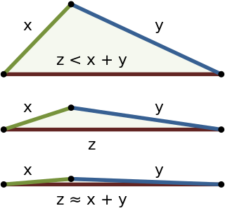
In mathematics, the triangle inequality states that for any triangle, the sum of the lengths of any two sides must be greater than or equal to the length of the remaining side. This statement permits the inclusion of degenerate triangles, but some authors, especially those writing about elementary geometry, will exclude this possibility, thus leaving out the possibility of equality. If x, y, and z are the lengths of the sides of the triangle, with no side being greater than z, then the triangle inequality states that
A mathematical symbol is a figure or a combination of figures that is used to represent a mathematical object, an action on mathematical objects, a relation between mathematical objects, or for structuring the other symbols that occur in a formula. As formulas are entirely constituted with symbols of various types, many symbols are needed for expressing all mathematics.
In mathematical analysis, Hölder's inequality, named after Otto Hölder, is a fundamental inequality between integrals and an indispensable tool for the study of Lp spaces.
In mathematics, a real-valued function is called convex if the line segment between any two distinct points on the graph of the function lies above the graph between the two points. Equivalently, a function is convex if its epigraph is a convex set. In simple terms, a convex function graph is shaped like a cup , while a concave function's graph is shaped like a cap .
In mathematics, Jensen's inequality, named after the Danish mathematician Johan Jensen, relates the value of a convex function of an integral to the integral of the convex function. It was proved by Jensen in 1906, building on an earlier proof of the same inequality for doubly-differentiable functions by Otto Hölder in 1889. Given its generality, the inequality appears in many forms depending on the context, some of which are presented below. In its simplest form the inequality states that the convex transformation of a mean is less than or equal to the mean applied after convex transformation; it is a simple corollary that the opposite is true of concave transformations.
In mathematics, the inequality of arithmetic and geometric means, or more briefly the AM–GM inequality, states that the arithmetic mean of a list of non-negative real numbers is greater than or equal to the geometric mean of the same list; and further, that the two means are equal if and only if every number in the list is the same.
In mathematics, the rearrangement inequality states that for every choice of real numbers
In mathematics, a norm is a function from a real or complex vector space to the non-negative real numbers that behaves in certain ways like the distance from the origin: it commutes with scaling, obeys a form of the triangle inequality, and is zero only at the origin. In particular, the Euclidean distance in a Euclidean space is defined by a norm on the associated Euclidean vector space, called the Euclidean norm, the 2-norm, or, sometimes, the magnitude of the vector. This norm can be defined as the square root of the inner product of a vector with itself.
In mathematics, Muirhead's inequality, named after Robert Franklin Muirhead, also known as the "bunching" method, generalizes the inequality of arithmetic and geometric means.
In mathematics, the logarithmic mean is a function of two non-negative numbers which is equal to their difference divided by the logarithm of their quotient. This calculation is applicable in engineering problems involving heat and mass transfer.
In probability theory and statistics, a stochastic order quantifies the concept of one random variable being "bigger" than another. These are usually partial orders, so that one random variable may be neither stochastically greater than, less than, nor equal to another random variable . Many different orders exist, which have different applications.
Anatoly Alexeyevich Karatsuba was a Russian mathematician working in the field of analytic number theory, p-adic numbers and Dirichlet series.
In mathematics, the Fortuin–Kasteleyn–Ginibre (FKG) inequality is a correlation inequality, a fundamental tool in statistical mechanics and probabilistic combinatorics, due to Cees M. Fortuin, Pieter W. Kasteleyn, and Jean Ginibre. Informally, it says that in many random systems, increasing events are positively correlated, while an increasing and a decreasing event are negatively correlated. It was obtained by studying the random cluster model.
In probability theory, concentration inequalities provide mathematical bounds on the probability of a random variable deviating from some value.
↑ Simovici, Dan A. & Djeraba, Chabane (2008). "Partially Ordered Sets". Mathematical Tools for Data Mining: Set Theory, Partial Orders, Combinatorics. Springer. ISBN9781848002012.
↑ Brian W. Kernighan and Dennis M. Ritchie (Apr 1988). The C Programming Language. Prentice Hall Software Series (2nded.). Englewood Cliffs/NJ: Prentice Hall. ISBN0131103628. Here: Sect.A.7.9 Relational Operators, p.167: Quote: "a<b<c is parsed as (a<b)<c"
Hardy, G., Littlewood J. E., Pólya, G. (1999). Inequalities. Cambridge Mathematical Library, Cambridge University Press. ISBN0-521-05206-8.{{cite book}}: CS1 maint: multiple names: authors list (link)
Beckenbach, E. F., Bellman, R. (1975). An Introduction to Inequalities. Random House Inc. ISBN0-394-01559-2.{{cite book}}: CS1 maint: multiple names: authors list (link)
Grinshpan, A. Z. (2005), "General inequalities, consequences, and applications", Advances in Applied Mathematics, 34 (1): 71–100, doi:10.1016/j.aam.2004.05.001
This page is based on this Wikipedia article Text is available under the CC BY-SA 4.0 license; additional terms may apply. Images, videos and audio are available under their respective licenses.