Atmospheric dispersion modeling

Last updated

Atmospheric dispersion modeling is the mathematical simulation of how air pollutants disperse in the ambient atmosphere. It is performed with computer programs that include algorithms to solve the mathematical equations that govern the pollutant dispersion. The dispersion models are used to estimate the downwind ambient concentration of air pollutants or toxins emitted from sources such as industrial plants, vehicular traffic or accidental chemical releases. They can also be used to predict future concentrations under specific scenarios (i.e. changes in emission sources). Therefore, they are the dominant type of model used in air quality policy making. They are most useful for pollutants that are dispersed over large distances and that may react in the atmosphere. For pollutants that have a very high spatio-temporal variability (i.e. have very steep distance to source decay such as black carbon) and for epidemiological studies statistical land-use regression models are also used.

Contents

Dispersion models are important to governmental agencies tasked with protecting and managing the ambient air quality. The models are typically employed to determine whether existing or proposed new industrial facilities are or will be in compliance with the National Ambient Air Quality Standards (NAAQS) in the United States and other nations. The models also serve to assist in the design of effective control strategies to reduce emissions of harmful air pollutants. During the late 1960s, the Air Pollution Control Office of the U.S. EPA initiated research projects that would lead to the development of models for the use by urban and transportation planners. [1] A major and significant application of a roadway dispersion model that resulted from such research was applied to the Spadina Expressway of Canada in 1971.

Air dispersion models are also used by public safety responders and emergency management personnel for emergency planning of accidental chemical releases. Models are used to determine the consequences of accidental releases of hazardous or toxic materials, Accidental releases may result in fires, spills or explosions that involve hazardous materials, such as chemicals or radionuclides. The results of dispersion modeling, using worst case accidental release source terms and meteorological conditions, can provide an estimate of location impacted areas, ambient concentrations, and be used to determine protective actions appropriate in the event a release occurs. Appropriate protective actions may include evacuation or shelter in place for persons in the downwind direction. At industrial facilities, this type of consequence assessment or emergency planning is required under the U.S. Clean Air Act (CAA) codified in Part 68 of Title 40 of the Code of Federal Regulations.

The dispersion models vary depending on the mathematics used to develop the model, but all require the input of data that may include:

Many of the modern, advanced dispersion modeling programs include a pre-processor module for the input of meteorological and other data, and many also include a post-processor module for graphing the output data and/or plotting the area impacted by the air pollutants on maps. The plots of areas impacted may also include isopleths showing areas of minimal to high concentrations that define areas of the highest health risk. The isopleths plots are useful in determining protective actions for the public and responders.

The atmospheric dispersion models are also known as atmospheric diffusion models, air dispersion models, air quality models, and air pollution dispersion models.

Atmospheric layers

Discussion of the layers in the Earth's atmosphere is needed to understand where airborne pollutants disperse in the atmosphere. The layer closest to the Earth's surface is known as the troposphere . It extends from sea-level to a height of about 18 km (11 mi) and contains about 80 percent of the mass of the overall atmosphere. The stratosphere is the next layer and extends from 18 km (11 mi) to about 50 km (31 mi). The third layer is the mesosphere which extends from 50 km (31 mi) to about 80 km (50 mi). There are other layers above 80 km, but they are insignificant with respect to atmospheric dispersion modeling.

The lowest part of the troposphere is called the atmospheric boundary layer (ABL) or the planetary boundary layer (PBL) . The air temperature of the atmosphere decreases with increasing altitude until it reaches what is called an inversion layer (where the temperature increases with increasing altitude) that caps the Convective Boundary Layer, typically to about 1.5 to 2 km (0.93 to 1.24 mi) in height. The upper part of the troposphere (i.e., above the inversion layer) is called the free troposphere and it extends up to the tropopause (the boundary in the Earth's atmosphere between the troposphere and the stratosphere). In tropical and mid-latitudes during daytime, the Free convective layer can comprise the entire troposphere, which is up to 10 to 18 km (6.2 to 11.2 mi) in the Intertropical convergence zone.

The ABL is of the most important with respect to the emission, transport and dispersion of airborne pollutants. The part of the ABL between the Earth's surface and the bottom of the inversion layer is known as the mixing layer. Almost all of the airborne pollutants emitted into the ambient atmosphere are transported and dispersed within the mixing layer. Some of the emissions penetrate the inversion layer and enter the free troposphere above the ABL.

In summary, the layers of the Earth's atmosphere from the surface of the ground upwards are: the ABL made up of the mixing layer capped by the inversion layer; the free troposphere; the stratosphere; the mesosphere and others. Many atmospheric dispersion models are referred to as boundary layer models because they mainly model air pollutant dispersion within the ABL. To avoid confusion, models referred to as mesoscale models have dispersion modeling capabilities that extend horizontally up to a few hundred kilometres. It does not mean that they model dispersion in the mesosphere.

Gaussian air pollutant dispersion equation

The technical literature on air pollution dispersion is quite extensive and dates back to the 1930s and earlier. One of the early air pollutant plume dispersion equations was derived by Bosanquet and Pearson. [2] Their equation did not assume Gaussian distribution nor did it include the effect of ground reflection of the pollutant plume.

Sir Graham Sutton derived an air pollutant plume dispersion equation in 1947 [3] which did include the assumption of Gaussian distribution for the vertical and crosswind dispersion of the plume and also included the effect of ground reflection of the plume.

Under the stimulus provided by the advent of stringent environmental control regulations, there was an immense growth in the use of air pollutant plume dispersion calculations between the late 1960s and today. A great many computer programs for calculating the dispersion of air pollutant emissions were developed during that period of time and they were called "air dispersion models". The basis for most of those models was the Complete Equation For Gaussian Dispersion Modeling Of Continuous, Buoyant Air Pollution Plumes shown below: [4] [5]

where: 
= crosswind dispersion parameter
 =
= vertical dispersion parameter =
= vertical dispersion with no reflections
 =
= vertical dispersion for reflection from the ground
 =
= vertical dispersion for reflection from an inversion aloft
 =


= concentration of emissions, in g/m³, at any receptor located:
       x meters downwind from the emission source point
       y meters crosswind from the emission plume centerline
       z meters above ground level
= source pollutant emission rate, in g/s
= horizontal wind velocity along the plume centerline, m/s
= height of emission plume centerline above ground level, in m
= vertical standard deviation of the emission distribution, in m
= horizontal standard deviation of the emission distribution, in m
= height from ground level to bottom of the inversion aloft, in m
= the exponential function

The above equation not only includes upward reflection from the ground, it also includes downward reflection from the bottom of any inversion lid present in the atmosphere.

The sum of the four exponential terms in converges to a final value quite rapidly. For most cases, the summation of the series with m = 1, m = 2 and m = 3 will provide an adequate solution.

and are functions of the atmospheric stability class (i.e., a measure of the turbulence in the ambient atmosphere) and of the downwind distance to the receptor. The two most important variables affecting the degree of pollutant emission dispersion obtained are the height of the emission source point and the degree of atmospheric turbulence. The more turbulence, the better the degree of dispersion.

Equations [6] [7] for and are:

(x) = exp(Iy + Jyln(x) + Ky[ln(x)]2)

(x) = exp(Iz + Jzln(x) + Kz[ln(x)]2)

(units of , and , and x are in meters)

CoefficientABCDEF
Iy-1.104-1.634-2.054-2.555-2.754-3.143
Jy0.98781.03501.02311.04231.01061.0148
Ky-0.0076-0.0096-0.0076-0.0087-0.0064-0.0070
Iz4.679-1.999-2.341-3.186-3.783-4.490
Jz-1.71720.87520.94771.17371.30101.4024
Kz0.27700.0136-0.0020-0.0316-0.0450-0.0540

The classification of stability class is proposed by F. Pasquill. [8] The six stability classes are referred to: A-extremely unstable B-moderately unstable C-slightly unstable D-neutral E-slightly stable F-moderately stable

The resulting calculations for air pollutant concentrations are often expressed as an air pollutant concentration contour map in order to show the spatial variation in contaminant levels over a wide area under study. In this way the contour lines can overlay sensitive receptor locations and reveal the spatial relationship of air pollutants to areas of interest.

Whereas older models rely on stability classes (see air pollution dispersion terminology) for the determination of and , more recent models increasingly rely on the Monin-Obukhov similarity theory to derive these parameters.

Briggs plume rise equations

The Gaussian air pollutant dispersion equation (discussed above) requires the input of H which is the pollutant plume's centerline height above ground level—and H is the sum of Hs (the actual physical height of the pollutant plume's emission source point) plus ΔH (the plume rise due to the plume's buoyancy).

Visualization of a buoyant Gaussian air pollutant dispersion plume Gaussian Plume (SVG).svg
Visualization of a buoyant Gaussian air pollutant dispersion plume

To determine ΔH, many if not most of the air dispersion models developed between the late 1960s and the early 2000s used what are known as the Briggs equations. G.A. Briggs first published his plume rise observations and comparisons in 1965. [9] In 1968, at a symposium sponsored by CONCAWE (a Dutch organization), he compared many of the plume rise models then available in the literature. [10] In that same year, Briggs also wrote the section of the publication edited by Slade [11] dealing with the comparative analyses of plume rise models. That was followed in 1969 by his classical critical review of the entire plume rise literature, [12] in which he proposed a set of plume rise equations which have become widely known as "the Briggs equations". Subsequently, Briggs modified his 1969 plume rise equations in 1971 and in 1972. [13] [14]

Briggs divided air pollution plumes into these four general categories:

Briggs considered the trajectory of cold jet plumes to be dominated by their initial velocity momentum, and the trajectory of hot, buoyant plumes to be dominated by their buoyant momentum to the extent that their initial velocity momentum was relatively unimportant. Although Briggs proposed plume rise equations for each of the above plume categories, it is important to emphasize that "the Briggs equations" which become widely used are those that he proposed for bent-over, hot buoyant plumes.

In general, Briggs's equations for bent-over, hot buoyant plumes are based on observations and data involving plumes from typical combustion sources such as the flue gas stacks from steam-generating boilers burning fossil fuels in large power plants. Therefore, the stack exit velocities were probably in the range of 20 to 100 ft/s (6 to 30 m/s) with exit temperatures ranging from 250 to 500 °F (120 to 260 °C).

A logic diagram for using the Briggs equations [4] to obtain the plume rise trajectory of bent-over buoyant plumes is presented below:

BriggsLogic.png
where: 
Δh= plume rise, in m
F = buoyancy factor, in m4s−3
x= downwind distance from plume source, in m
xf= downwind distance from plume source to point of maximum plume rise, in m
u= windspeed at actual stack height, in m/s
s = stability parameter, in s−2

The above parameters used in the Briggs' equations are discussed in Beychok's book. [4]

See also

Atmospheric dispersion models

List of atmospheric dispersion models provides a more comprehensive list of models than listed below. It includes a very brief description of each model.

Result of an atmospheric dispersion modeling using AERMOD Resultat de modelisation de dispersion atmospherique - Avizo Experts-Conseils.png
Result of an atmospheric dispersion modeling using AERMOD
2016 HYSPLIT map HYSPLITTrajectoriesforNewportStateParkpage72.jpg
2016 HYSPLIT map
3D dynamic FEM air pollution transport model - concentration field on ground level Vanadis a1 test.gif
3D dynamic FEM air pollution transport model - concentration field on ground level
3D dynamic FEM air pollution transport model - concentration field on perpendicular surface Vanadis a2 test.gif
3D dynamic FEM air pollution transport model - concentration field on perpendicular surface

Organizations

Others

Related Research Articles

<span class="mw-page-title-main">Troposphere</span> Lowest layer of Earths atmosphere

The troposphere is the lowest layer of the atmosphere of Earth. It contains 75% of the total mass of the planetary atmosphere and 99% of the total mass of water vapor and aerosols, and is where most weather phenomena occur. From the planetary surface of the Earth, the average height of the troposphere is 18 km in the tropics; 17 km in the middle latitudes; and 6 km in the high latitudes of the polar regions in winter; thus the average height of the troposphere is 13 km.

<span class="mw-page-title-main">Plume (fluid dynamics)</span> Column of one fluid moving through another

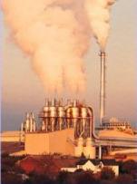
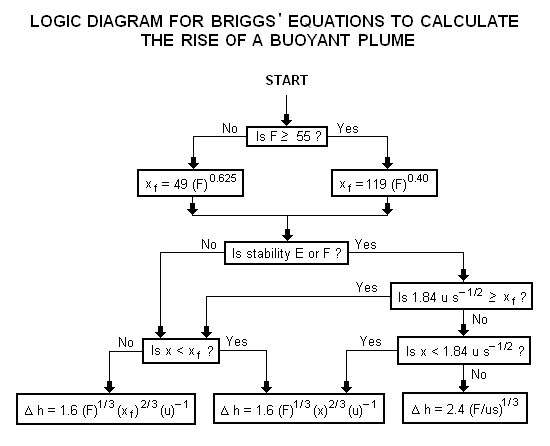
In hydrodynamics, a plume or a column is a vertical body of one fluid moving through another. Several effects control the motion of the fluid, including momentum (inertia), diffusion and buoyancy. Pure jets and pure plumes define flows that are driven entirely by momentum and buoyancy effects, respectively. Flows between these two limits are usually described as forced plumes or buoyant jets. "Buoyancy is defined as being positive" when, in the absence of other forces or initial motion, the entering fluid would tend to rise. Situations where the density of the plume fluid is greater than its surroundings, but the flow has sufficient initial momentum to carry it some distance vertically, are described as being negatively buoyant.

Various governmental agencies involved with environmental protection and with occupational safety and health have promulgated regulations limiting the allowable concentrations of gaseous pollutants in the ambient air or in emissions to the ambient air. Such regulations involve a number of different expressions of concentration. Some express the concentrations as ppmv and some express the concentrations as mg/m3, while others require adjusting or correcting the concentrations to reference conditions of moisture content, oxygen content or carbon dioxide content. This article presents a set of useful conversions and formulas for air dispersion modeling of atmospheric pollutants and for complying with the various regulations as to how to express the concentrations obtained by such modeling.

<span class="mw-page-title-main">Roadway air dispersion modeling</span> Study of air pollutant transport from a roadway

Roadway air dispersion modeling is the study of air pollutant transport from a roadway or other linear emitter. Computer models are required to conduct this analysis, because of the complex variables involved, including vehicle emissions, vehicle speed, meteorology, and terrain geometry. Line source dispersion has been studied since at least the 1960s, when the regulatory framework in the United States began requiring quantitative analysis of the air pollution consequences of major roadway and airport projects. By the early 1970s this subset of atmospheric dispersion models was being applied to real-world cases of highway planning, even including some controversial court cases.

The Atmospheric Dispersion Modelling Liaison Committee (ADMLC) is composed of representatives from government departments, agencies and private consultancies. The ADMLC's main aim is to review current understanding of atmospheric dispersion and related phenomena for application primarily in the authorization or licensing of pollutant emissions to the atmosphere from industrial, commercial or institutional sites.

Germany has an air pollution control regulation titled "Technical Instructions on Air Quality Control" and commonly referred to as the TA Luft.

The National Atmospheric Release Advisory Center (NARAC) is located at the University of California's Lawrence Livermore National Laboratory. It is a national support and resource center for planning, real-time assessment, emergency response, and detailed studies of incidents involving a wide variety of hazards, including nuclear, radiological, chemical, biological, and natural emissions.

CALPUFF is an advanced, integrated Lagrangian puff modeling system for the simulation of atmospheric pollution dispersion distributed by the Atmospheric Studies Group at TRC Solutions.

The ADMS 3 is an advanced atmospheric pollution dispersion model for calculating concentrations of atmospheric pollutants emitted both continuously from point, line, volume and area sources, or intermittently from point sources. It was developed by Cambridge Environmental Research Consultants (CERC) of the UK in collaboration with the UK Meteorological Office, National Power plc and the University of Surrey. The first version of ADMS was released in 1993. The version of the ADMS model discussed on this page is version 3 and was released in February 1999. It runs on Microsoft Windows. The current release, ADMS 5 Service Pack 1, was released in April 2013 with a number of additional features.

<span class="mw-page-title-main">AERMOD</span>

The AERMOD atmospheric dispersion modeling system is an integrated system that includes three modules:

NAME atmospheric pollution dispersion model was first developed by the UK's Met Office in 1986 after the nuclear accident at Chernobyl, which demonstrated the need for a method that could predict the spread and deposition of radioactive gases or material released into the atmosphere.

The following outline is provided as an overview of and topical guide to air pollution dispersion: In environmental science, air pollution dispersion is the distribution of air pollution into the atmosphere. Air pollution is the introduction of particulates, biological molecules, or other harmful materials into Earth's atmosphere, causing disease, death to humans, damage to other living organisms such as food crops, and the natural or built environment. Air pollution may come from anthropogenic or natural sources. Dispersion refers to what happens to the pollution during and after its introduction; understanding this may help in identifying and controlling it.

ISC3 (Industrial Source Complex) model is a popular steady-state Gaussian plume model which can be used to assess pollutant concentrations from a wide variety of sources associated with an industrial complex.

SAFE AIR is an advanced atmospheric pollution dispersion model for calculating concentrations of atmospheric pollutants emitted both continuously or intermittently from point, line, volume and area sources. It adopts an integrated Gaussian puff modeling system. SAFE AIR consists of three main parts: the meteorological pre-processor WINDS to calculate wind fields, the meteorological pre-processor ABLE to calculate atmospheric parameters and a lagrangian multisource model named P6 to calculate pollutant dispersion. SAFE AIR is included in the online Model Documentation System (MDS) of the European Environment Agency (EEA) and of the Italian Agency for the Protection of the Environment (APAT).

A chemical transport model (CTM) is a type of computer numerical model which typically simulates atmospheric chemistry and may give air pollution forecasting.

<span class="mw-page-title-main">Idealized greenhouse model</span> Mathematical estimate of planetary temperatures

The temperatures of a planet's surface and atmosphere are governed by a delicate balancing of their energy flows. The idealized greenhouse model is based on the fact that certain gases in the Earth's atmosphere, including carbon dioxide and water vapour, are transparent to the high-frequency solar radiation, but are much more opaque to the lower frequency infrared radiation leaving Earth's surface. Thus heat is easily let in, but is partially trapped by these gases as it tries to leave. Rather than get hotter and hotter, Kirchhoff's law of thermal radiation says that the gases of the atmosphere also have to re-emit the infrared energy that they absorb, and they do so, also at long infrared wavelengths, both upwards into space as well as downwards back towards the Earth's surface. In the long-term, the planet's thermal inertia is surmounted and a new thermal equilibrium is reached when all energy arriving on the planet is leaving again at the same rate. In this steady-state model, the greenhouse gases cause the surface of the planet to be warmer than it would be without them, in order for a balanced amount of heat energy to finally be radiated out into space from the top of the atmosphere.

Turbulent diffusion is the transport of mass, heat, or momentum within a system due to random and chaotic time dependent motions. It occurs when turbulent fluid systems reach critical conditions in response to shear flow, which results from a combination of steep concentration gradients, density gradients, and high velocities. It occurs much more rapidly than molecular diffusion and is therefore extremely important for problems concerning mixing and transport in systems dealing with combustion, contaminants, dissolved oxygen, and solutions in industry. In these fields, turbulent diffusion acts as an excellent process for quickly reducing the concentrations of a species in a fluid or environment, in cases where this is needed for rapid mixing during processing, or rapid pollutant or contaminant reduction for safety.

<span class="mw-page-title-main">Air pollutant concentrations</span>

Air pollutant concentrations, as measured or as calculated by air pollution dispersion modeling, must often be converted or corrected to be expressed as required by the regulations issued by various governmental agencies. Regulations that define and limit the concentration of pollutants in the ambient air or in gaseous emissions to the ambient air are issued by various national and state environmental protection and occupational health and safety agencies.

<span class="mw-page-title-main">History of numerical weather prediction</span> Aspect of meteorological history

The history of numerical weather prediction considers how current weather conditions as input into mathematical models of the atmosphere and oceans to predict the weather and future sea state has changed over the years. Though first attempted manually in the 1920s, it was not until the advent of the computer and computer simulation that computation time was reduced to less than the forecast period itself. ENIAC was used to create the first forecasts via computer in 1950, and over the years more powerful computers have been used to increase the size of initial datasets as well as include more complicated versions of the equations of motion. The development of global forecasting models led to the first climate models. The development of limited area (regional) models facilitated advances in forecasting the tracks of tropical cyclone as well as air quality in the 1970s and 1980s.

References

  1. Fensterstock, J.C. et al., "Reduction of air pollution potential through environmental planning" [ permanent dead link ], JAPCA, Vol.21, No.7, 1971.
  2. Bosanquet, C.H. and Pearson, J.L., "The spread of smoke and gases from chimneys", Trans. Faraday Soc., 32:1249, 1936
  3. Sutton, O.G., "The problem of diffusion in the lower atmosphere", QJRMS, 73:257, 1947 and "The theoretical distribution of airborne pollution from factory chimneys", QJRMS, 73:426, 1947
  4. 1 2 3 Beychok, Milton R. (2005). Fundamentals Of Stack Gas Dispersion (4th ed.). author-published. ISBN   0-9644588-0-2.
  5. Turner, D.B. (1994). Workbook of atmospheric dispersion estimates: an introduction to dispersion modeling (2nd ed.). CRC Press. ISBN   1-56670-023-X.
  6. Seinfeld, John H. (2006). "Chapter 18". Atmospheric chemistry and physics: from air pollution to climate change. Wiley. ISBN   9780471720171.
  7. Hanna, Steven (1982). "Handbook on Atmospheric Diffusion". U.S. Department of Energy Report.
  8. W, Klug (April 1984). Atmospheric Diffusion (3rd Edition). F. Pasquill and F. B. Smith. Ellis Horwood, (John Wiley & Sons) Chichester, 1983 (3rd ed.). New York: Quarterly Journal of the Royal Meteorological Society.
  9. Briggs, G.A., "A plume rise model compared with observations", JAPCA, 15:433–438, 1965
  10. Briggs, G.A., "CONCAWE meeting: discussion of the comparative consequences of different plume rise formulas", Atmos. Envir., 2:228–232, 1968
  11. Slade, D.H. (editor), "Meteorology and atomic energy 1968", Air Resources Laboratory, U.S. Dept. of Commerce, 1968
  12. Briggs, G.A., "Plume Rise", USAEC Critical Review Series, 1969
  13. Briggs, G.A., "Some recent analyses of plume rise observation", Proc. Second Internat'l. Clean Air Congress, Academic Press, New York, 1971
  14. Briggs, G.A., "Discussion: chimney plumes in neutral and stable surroundings", Atmos. Envir., 6:507–510, 1972

Further reading

Books

Introductory
Advanced
  • Arya, S. Pal (1998). Air Pollution Meteorology and Dispersion (1st ed.). Oxford University Press. ISBN   0-19-507398-3.
  • Barrat, Rod (2001). Atmospheric Dispersion Modelling (1st ed.). Earthscan Publications. ISBN   1-85383-642-7.
  • Colls, Jeremy (2002). Air Pollution (1st ed.). Spon Press (UK). ISBN   0-415-25565-1.
  • Cooper JR, Randle K, Sokh RG (2003). Radioactive Releases in the Environment (1st ed.). John Wiley & Sons. ISBN   0-471-89924-0.
  • European Process Safety Centre (1999). Atmospheric Dispersion (1st ed.). Rugby: Institution of Chemical Engineers. ISBN   0-85295-404-2.
  • Godish, Thad (2003). Air Quality (4th ed.). CRC Press. ISBN   1-56670-586-X.
  • Hanna, S.R. & Drivas, D. G. (1996). Guidelines for Use of Vapor Cloud Dispersion Models (2nd ed.). Wiley-American Institute of Chemical Engineers. ISBN   0-8169-0702-1.
  • Hanna, S. R. & Strimaitis, D. G. (1989). Workbook of Test Cases for Vapor Cloud Source Dispersion Models (1st ed.). Center for Chemical Process Safety, American Institute of Chemical Engineers. ISBN   0-8169-0455-3.
  • Hanna, S. R. & Britter, R.E. (2002). Wind Flow and Vapor Cloud Dispersion at Industrial and Urban Sites (1st ed.). Wiley-American Institute of Chemical Engineers. ISBN   0-8169-0863-X.
  • Perianez, Raul (2005). Modelling the dispersion of radionuclides in the marine environment : an introduction (1st ed.). Springer. ISBN   3-540-24875-7.
  • Pielke, Roger A. (2001). Mesoscale Modeling (2nd ed.). Elsevier. ISBN   0-12-554766-8.
  • Zannetti, P. (1990). Air pollution modeling : theories, computational methods, and available software. Van Nostrand Reinhold. ISBN   0-442-30805-1.

Proceedings

  • Forago I, Georgiev K, Havasi A, eds. (2004). Advances in Air Pollution Modeling for Environmental Security (NATO Workshop). Springer, 2005. ISSN   0957-4352.
  • Kretzschmar JG, Cosemans G, eds. (1996). Harmonization within atmospheric dispersion modelling for regulatory purposes (4th Workshop). International Journal of Environment and Pollution, vol. 8 no. 3–6, Interscience Enterprises, 1997. ISSN   0957-4352.
  • Bartzis, J G., ed. (1998). Harmonization within atmospheric dispersion modelling for regulatory purposes (5th Workshop). International Journal of Environment and Pollution, vol. 14 no. 1–6, Interscience Enterprises, 2000. ISSN   0957-4352.
  • Coppalle, A., ed. (1999). Harmonization within atmospheric dispersion modelling for regulatory purposes (6th Workshop). International Journal of Environment and Pollution, vol. 16 no. 1–6, Inderscience Enterprises, 2001. ISSN   0957-4352.
  • Batchvarova, E., ed. (2002). Harmonization within atmospheric dispersion modelling for regulatory purposes (8th Workshop). International Journal of Environment and Pollution, vol. 20 no. 1–6, Inderscience Enterprises, 2003. ISSN   0957-4352.
  • Suppan, P., ed. (2004). Harmonization within atmospheric dispersion modelling for regulatory purposes (8th Workshop). International Journal of Environment and Pollution, vol. 24 no. 1–6 and vol.25 no. 1–6, Inderscience Enterprises, 2005. ISSN   0957-4352.
  • Zannetti, P., ed. (1993). International Conference on Air Pollution (1st, Mexico City). Computational Mechanics, 1993. ISBN   1-56252-146-2.
  • De Wispelaere, C., ed. (1980). International Technical Meeting on Air Pollution Modeling and Its Application (11th). Plenum Press, 1981. ISBN   0-306-40820-1.
  • De Wispelaere, C., ed. (1982). International Technical Meeting on Air Pollution Modeling and Its Application (13th). NATO Committee on the Challenges of Modern Society [by] Plenum Press, 1984. ISBN   0-306-41491-0.
  • Gryning, S.; Schiermeir, F.A., eds. (1995). International Technical Meeting on Air Pollution Modeling and Its Application (21st). NATO Committee on the Challenges of Modern Society [by] Plenum Press, 1996. ISBN   0-306-45381-9.
  • Gryning, S.; Chaumerliac, N., eds. (1997). International Technical Meeting on Air Pollution Modeling and Its Application (22nd). NATO Committee on the Challenges of Modern Society [by] Plenum Press, 1998. ISBN   0-306-45821-7.
  • Gryning, S.; Batchvarova, E., eds. (1998). International Technical Meeting on Air Pollution Modeling and Its Application (23rd). NATO Committee on the Challenges of Modern Society [by] Kluwer Academic/Plenum Press, 2000. ISBN   0-306-46188-9.
  • Gryning, S.; Schiermeir, F.A., eds. (2000). International Technical Meeting on Air Pollution Modeling and Its Application (24th). NATO Committee on the Challenges of Modern Society [by] Kluwer Academic, 2001. ISBN   0-306-46534-5.
  • Borrego, C.; Schayes, G., eds. (2000). International Technical Meeting on Air Pollution Modeling and Its Application (25th). NATO Committee on the Challenges of Modern Society [by] Kluwer Academic, 2002. ISBN   0-306-47294-5.
  • Borrego, C.; Incecik, S., eds. (2003). International Technical Meeting on Air Pollution Modeling and Its Application (26th). NATO Committee on the Challenges of Modern Society [by] Kluwer Academic/Plenum Press, 2004. ISBN   0-306-48464-1.
  • Committee on the Atmospheric Dispersion of Hazardous Material Releases, National Research Council, ed. (2002). Tracking and Predicting the Atmospheric Dispersion of Hazardous Material Releases (Workshop). National Academies Press, 2003. ISBN   0-309-08926-3.

Guidance