Biological motion perception

Biological motion perception is the act of perceiving the fluid unique motion of a biological agent. The phenomenon was first documented by Swedish perceptual psychologist, Gunnar Johansson, in 1973. ^[1] There are many brain areas involved in this process, some similar to those used to perceive faces. While humans complete this process with ease, from a computational neuroscience perspective there is still much to be learned as to how this complex perceptual problem is solved. One tool which many research studies in this area use is a display stimuli called a point light walker. Point light walkers are coordinated moving dots that simulate biological motion in which each dot represents specific joints of a human performing an action.

Currently a large topic of research, many different models of biological motion/perception have been proposed. The following models have shown that both form and motion are important components of biological motion perception. However, to what extent each of the components play is contrasted upon the models.

Neuroanatomy

Research in this area seeks to identify the specific brain regions or circuits responsible for processing the information which the visual system perceives in the world. And in this case, specifically recognizing motion created by biological agents.

Single Cell Recording

The most precise research is done using single-cell recordings in the primate brain. This research has yielded areas important to motion perception in primates such as area MT (middle temporal visual area), also referred to as V5, and area MST (medial superior temporal area). These areas contain cells characterized as direction cells, expansion/contraction cells, and rotation cells, which react to certain classes of movement. ^{[2] [3] [4]}

Neuroimaging

Additionally, research on human participants is being conducted as well. While single-cell recording is not conducted on humans, this research uses neuroimaging methods such as fMRI, PET, EEG/ERP to collect information on what brain areas become active when executing biological motion perception tasks, such as viewing point light walker stimuli. Areas uncovered from this type of research are the dorsal visual pathway, extrastriate body area, fusiform gyrus, superior temporal sulcus, and premotor cortex. The dorsal visual pathway (sometimes referred to as the "where" pathway), as contrasted with the ventral visual pathway ("what" pathway), has been shown to play a significant role in the perception of motion cues. While the ventral pathway is more responsible for form cues. ^{[5] [6] [7] [8] [9] [10]}

Neuropsychological Damage

Valuable information can also be learned from cases where a patient has suffered from some sort of neurological damage and consequently loses certain functionalities of neural processing. One patient with bilateral lesions that included the human homologue of area MT, lost their ability to see biological motion when the stimulus was embedded in noise, a task which the average observer is able to complete. Another study on stroke patients sustaining lesions to their superior temporal and premotor frontal areas showed deficits in their processing of biological motion stimuli, thereby implicating these areas as important to that perception process. A case study conducted on a patient with bilateral lesions involving the posterior visual pathways and effecting the lateral parietal-temporal-occipital cortex struggled with early motion tasks, and yet was able to perceive the biological motion of a point light walker, a higher-order task. This may be due to the fact that area V3B and area KO were still intact, suggesting their possible roles in biological motion perception. ^{[11] [12] [13]}

Biological Motion Perception Models

Cognitive Model of Biological Motion Form (Lange & Lappe, 2006)

^[14]

Background

The relative roles of form cues compared to motion cues in the process of perceiving biological motion is unclear. Previous research has not untangled the circumstances under which local motion cues are needed or only additive. This model looks at how form-only cues can replicate psychophysical results of biological motion perception.

Model

Template Creation

Same as below. See 2.2.2 Template Generation

Stage 1

The first stage compares stimulus images to the assumed library of upright human walker templates in memory. Each dot in a given stimulus frame is compared to the nearest limb location on a template and these combined, weighted distances are outputted by the function:

${\displaystyle F_{tc}(t)=\sum _{i=1}^{n}e^{\left({\frac {(\mu _{tc}-p_{i}(t))^{2}}{2X\sigma }}\right)}}$

where ${\displaystyle p_{i}}$ gives the position of a particular stimulus dot and ${\displaystyle \mu _{tc}}$ represents the nearest limb position in the template. ${\displaystyle \sigma }$ represents the size of the receptor field to adjust for the size of the stimulus figure.

The best fitting template was then selected by a winner-takes-all mechanism and entered into a leaky integrator:

${\displaystyle \tau {\frac {\delta u_{1,2}(t)}{\delta t}}=-u_{1,2}+i_{1,2}+w_{+}f(u_{1,2}(t))-w_{-}f(u_{2,1}(t))}$

where ${\displaystyle w_{+}}$ and ${\displaystyle w_{-}}$ are the weights for lateral excitation and inhibition, respectively, and the activities ${\displaystyle u_{1,2}}$ provide the left/right decision for which direction the stimulus is facing.

Stage 2

The second stage attempts to use the temporal order of the stimulus frames to change the expectations of what frame would be coming next. The equation

${\displaystyle \tau {\frac {\delta v_{1,2}(t)}{\delta t}}=-v_{1,2}(t)+w_{m,n}u(t)}$

takes into account bottom-up input from stage 1 ${\displaystyle (u)}$, the activities in decision stage 2 for the possible responses ${\displaystyle (v_{1,2})}$, and weights the difference between selected frame ${\displaystyle n}$ and previous frame ${\displaystyle m}$.

Implications

This model highlights the abilities of form-related cues to detect biological motion and orientation in a neurologically feasible model. The results of the Stage 1 model showed that all behavioral data could be replicated by using form information alone - global motion information was not necessary to detect figures and their orientation. This model shows the possibility of the use of form cues, but can be criticized for a lack of ecological validity. Humans do not detect biological figures in static environments and motion is an inherent aspect in upright figure recognition.

Action Recognition by Motion Detection in Posture Space (Theusner, Lussanet, and Lappe, 2014)

Overview

Old models of biological motion perception are concerned with tracking joint and limb motion relative to one another over time. ^[1] However, recent experiments in biological motion perception have suggested that motion information is unimportant for action recognition. ^[15] This model shows how biological motion may be perceived from sequences of posture recognition, rather than from the direct perception of motion information. An experiment was conducted to test the validity of this model, in which subjects are presented moving point-light and stick-figure walking stimuli. Each frame of the walking stimulus is matched to a posture template, the progression of which is recorded on a 2D posture–time plot that implies motion recognition.

Posture Model

Template Generation

Posture templates for stimulus matching were constructed with motion tracking data from nine people walking. ^[16] 3D coordinates of the twelve major joints (feet, knees, hips, hands, elbows, and shoulders) were tracked and interpolated between to generate limb motion. Five sets of 2D projections were created: leftward, frontward, rightward, and the two 45° intermediate orientations. Finally, projections of the nine walkers were normalized for walking speed (1.39 seconds at 100 frames per cycle), height, and hip location in posture space. One of the nine walkers was chosen as the walking stimulus, and the remaining eight were kept as templates for matching.

Template Matching

Template matching is computed by simulating posture selective neurons as described by ^[17] A neuron is excited by similarity to a static frame of the walker stimulus. For this experiment, 4,000 neurons were generated (8 walkers times 100 frames per cycle times 5 2D projections). A neuron's similarity to a frame of the stimulus is calculated as follows:

${\displaystyle R_{\psi }(t)=\sum _{i=1}^{N}\exp \left(-{\frac {\left|(x_{i}(t),y_{i}(t))-(\mathrm {X} _{i},_{\psi },\mathrm {P} _{i},_{\psi })\right\vert ^{2}}{2\cdot \sigma }}\right)}$

where ${\displaystyle (x_{i},y_{i})}$ describe a stimulus point and ${\displaystyle (c_{i},r_{i})}$ describe the limb location at time ${\displaystyle t}$; ${\displaystyle \psi }$ describes the preferred posture; ${\displaystyle R}$ describes a neuron's response to a stimulus of ${\displaystyle N}$ points; and ${\displaystyle \sigma }$ describes limb width.

Response Simulation

The neuron most closely resembling the posture of the walking stimulus changes over time. The neural activation pattern can be graphed in a 2D plot, called a posture-time plot. Along the x axis, templates are sorted chronologically according to a forward walking pattern. Time progresses along the y axis with the beginning corresponding to the origin. The perception of forward walking motion is represented as a line with a positive slope from the origin, while backward walking is conversely represented as a line with a negative slope.

Motion Model

Motion Detection in Posture Space

The posture-time plots used in this model follow the established space-time plots used for describing object motion. ^[18] Space-time plots with time at the y axis and the spatial dimension at the x axis, define velocity of an object by the slope of the line. Information about an object's motion can be detected by spatio-temporal filters. ^{[19] [20]} In this biological motion model, motion is detected similarly but replaces the spatial dimension for posture space along the x axis, and body motion is detected by using posturo-temporal filters rather than spatio-temporal filters.

Posturo-Temporal Filters

Neural responses are first normalized as described by ^[21]

${\displaystyle \nu _{\psi }(t)={\frac {R_{\psi }(t)-{\bar {R}}}{\bar {R}}}}$

where ${\displaystyle R_{y}(t)}$ describes the neural response; ${\displaystyle _{\psi }}$ describes the preferred posture at time ${\displaystyle t}$; ${\displaystyle {\bar {R}}}$ describes the mean neural response over all neurons over ${\displaystyle t}$; and ${\displaystyle n_{y}(t)}$ describes the normalized response. The filters are defined for forward and backward walking (${\displaystyle g^{f},g^{b}}$ respectively). The response of the posturo-temporal filter is described

${\displaystyle r_{\psi }(\tau )=\sum _{t=0ms}^{\tau }\sum _{p=1}^{100}g_{\tau ,\psi }(t,p)\cdot \nu _{\psi }(t)}$

where ${\displaystyle r}$ is the response of the filter at time ${\displaystyle \tau }$; and ${\displaystyle p}$ describes the posture dimension. The response of the filter is normalized by

${\displaystyle N_{\psi }(\tau )=\max \left[\left({\frac {r_{\psi }(\tau )}{\sum _{t}\sum _{p}g_{\tau ,\psi }(t,p)^{2}}}\right),0\right]}$

where ${\displaystyle N}$ describes the response of the neuron selecting body motion. Finally, body motion is calculated by

${\displaystyle \varepsilon _{\psi }(\tau )=N_{\psi }^{F}(\tau )^{2}-N_{\psi }^{B}(\tau )^{2}}$

where ${\displaystyle \varepsilon }$ describes body motion energy.

Critical Features for the Recognition of Biological Motion (Casille and Giese, 2005)

Statistical Analysis and Psychophysical Experiments

The following model suggests that biological motion recognition could be accomplished through the extraction of a single critical feature: dominant local optic flow motion. These following assumptions were brought about from results of both statistical analysis and psychophysical experiments. ^[22]

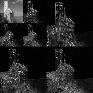
First, Principal component analysis was done on full body 2d walkers and point light walkers. The analysis found that dominant local optic flow features are very similar in both full body 2d stimuli and point light walkers (Figure 1). ^[22] Since subjects can recognize biological motion upon viewing a point light walker, then the similarities between these two stimuli may highlight critical features needed for biological motion recognition.

Through psychophysical experiments, it was found that subjects could recognize biological motion using a CFS stimulus which contained opponent motion in the horizontal direction but randomly moving dots in the horizontal direction (Figure 2). ^[22] Because of the movement of the dots, this stimulus could not be fit to a human skeleton model suggesting that biological motion recognition may not heavily rely on form as a critical feature. Also, the psychophysical experiments showed that subjects similarly recognize biological motion for both the CFS stimulus and SPS, a stimulus in which dots of the point light walker were reassigned to different positions within the human body shape for every nth frame thereby highlights the importance of form vs the motion (Fig.1.). ^[23] The results of the following psychophysical experiments show that motion is a critical feature that could be used to recognize biological motion.

The following statistical analysis and psychophysical experiments highlight the importance of dominant local motion patterns in biological motion recognition. Furthermore, due to the ability of subjects to recognize biological motion given the CFS stimulus, it is postulated that horizontal opponent motion and coarse positional information is important for recognition of biological motion.

Model

The following model contains detectors modeled from existing neurons that extracts motion features with increasing complexity. (Figure 4). ^[22]

Detectors of Local Motion

These detectors detect different motion directions and are modeled from neurons in monkey V1/2 and area MT ^[24] The output of the local motion detectors are the following:

${\displaystyle G_{p}(x)=H(v(x),v_{1},v_{2})\cdot b(\theta ,\theta _{p})}$

where ${\displaystyle x}$ is the position with preferred direction ${\displaystyle \theta _{p},}$, ${\displaystyle v}$ is the velocity, ${\displaystyle \theta }$ is the direction, and ${\displaystyle H}$ is the rectangular speed tuning function such that

${\displaystyle H(v,v_{1},v_{2})=1}$ for ${\displaystyle v_{1}<v<v_{2}}$ and ${\displaystyle H(v,v_{1},v_{2})=0}$ otherwise.

The direction-tuning of motion energy detectors are given by

${\displaystyle b(\theta ,\theta _{p})=\left\{\left({\frac {1}{2}}\right)\left[\ 1+cos(\theta ,\theta _{p})\right]\ \right\}^{q}}$

where ${\displaystyle q}$ is a parameter that determines width of direction tuning function. (q=2 for simulation).

Neural detectors for opponent motion selection

The following neural detectors are used to detect horizontal and vertical opponent motion due by pooling together the output of previous local motion energy detectors into two adjacent subfields. Local motion detectors that have the same direction preference are combined into the same subfield. These detectors were modeled after neurons sensitive to opponent motion such as the ones in MT and medial superior temporal (MST). ^{[25] [26]} Also, KO/V3B has been associated with processing edges, moving objects, and opponent motion. Patients with damage to dorsal pathway areas but an intact KO/V3B, as seen in patient AF can still perceive biological motion. ^[27]

The output for these detectors are the following:

${\displaystyle o_{l}(x)={\sqrt {max(g_{p}(x_{i}))max(g_{r}(x_{j}))}}}$

where ${\displaystyle x}$ is the position the output is centered at, direction preferences ${\displaystyle p}$ and ${\displaystyle r}$, and ${\displaystyle i,j}$ signify spatial positions of two subfields.

The final output of opponent motion detector is given as

${\displaystyle o_{l}(x)=max(o_{l}(x_{k}))}$

where output is the pooled responses of detectors of type ${\displaystyle l}$ at ${\displaystyle x_{k}}$ different spatial positions.

Detectors of optic flow patterns

Each detector looks at one frame of a training stimulus and compute an instantaneous optic flow field for that particular frame. These detectors model neurons in Superior temporal sulcus ^[28] and Fusiform face area ^[29]

The input of these detectors is arranged from vector u and are comprised from the previous opponent motion detectors' responses. The output is the following:

${\displaystyle G(u)=e^{(u-u_{0})^{T}C(u-u_{0})}}$

such that ${\displaystyle u_{0}}$ is the center of the radial basis function for each neuron and ${\displaystyle C}$ is a diagonal matrix which contains elements that have been set during training and correspond to vector u. These elements equal zero if the variance over training doesn't exceed a certain threshold. Otherwise, these elements equal the inverse of variance.

Since recognition of biological motion is dependent on the sequence of activity, the following model is sequence selective. The activity of the optic flow pattern neuron is modeled by the following equation of

${\displaystyle \tau H_{k}^{l}(t)=-H_{k}^{l}(t)+\sum _{m}w(k-m)f(H_{k}^{l}(t)+G_{k}^{l}(t))}$

in which ${\displaystyle k}$ is a specific frame in the ${\displaystyle l}$-th training sequence, ${\displaystyle \tau }$ is the time constant.${\displaystyle f(H)}$ a threshold function, ${\displaystyle w(m)}$ is an asymmetric interaction kernel, and ${\displaystyle G_{k}^{l}(t)}$ is obtained from the previous section.

Detectors of complete biological motion patterns The following detectors sum the output of the optic flow pattern detectors in order to selectively activate for whole movement patterns (e.g. walking right vs. walking left). These detectors model similar neurons that optic flow pattern detectors model:

Superior temporal sulcus ^[28] and Fusiform face area ^[29]

The input of these detectors are the activity of the optic flow motion detectors, ${\displaystyle H_{l}^{l}(t)}$. The output of these detectors are the following:

${\displaystyle \tau _{s}P^{l}(t)=-P^{l}(t)+\sum _{k}H_{l}^{l}(t)}$

such that ${\displaystyle P^{l}(t)}$ is the activity of the complete biological motion pattern detector in response to pattern type ${\displaystyle l}$ (e.g. walking to the left), ${\displaystyle \tau _{s}}$ equals the time constant (used 150 ms in simulation), and ${\displaystyle H_{k}^{l}(t)}$ equals the activity of optic flow pattern detector at kth frame in sequence l.

Testing the model

Using correct determination of walking direction of both the CFS and SPS stimulus, the model was able to replicate similar results as the psychophysical experiments. (could determine walking direction of CFS and SPS stimuli and increasing correct with increasing number of dots). It is postulated that recognition of biological motion is made possible by the opponent horizontal motion information that is present in both the CFS and SPS stimuli.

External links

Demo of point light walker:

References:

1. 1 2 Johansson (1973). "Visual perception of biological motion and a model for its analysis". Perception & Psychophysics. 14 (2): 201–214. doi: 10.3758/bf03212378 .
2. Born, Bradley (2005). "Structure and Function of Visual Area MT". Annual Review of Neuroscience. 28: 157–189. doi:10.1146/annurev.neuro.26.041002.131052. PMID   16022593.
3. Tanaka K, Saito H (1989). "Analysis of Motion of the Visual Field by Direction, Expansion/Contraction, and Rotation Cells Clustered in the Dorsal Part of the Medial Superior Temporal Area of the Macaque Monkey". Journal of Neurophysiology. 62 (3): 626–641. doi:10.1152/jn.1989.62.3.626. PMID   2769351. S2CID   5795874.
4. van Essen and Gallant (1994). "Neural Mechanisms of Form and Motion Processing in the Primate Visual System". Neuron. 13 (1): 1–10. doi:10.1016/0896-6273(94)90455-3. PMID   8043270. S2CID   17256399.
5. Grossman; et al. (2000). "Brain Areas Involved in the Perception of Biological Motion". Journal of Cognitive Neuroscience. 12 (5): 711–720. CiteSeerX   10.1.1.138.1319 . doi:10.1162/089892900562417. PMID   11054914. S2CID   15679202.
6. Ptito; et al. (2003). "Separate neural pathways for contour and biological-motion cues in motion-defined animal shapes". NeuroImage. 19 (2): 246–252. doi:10.1016/s1053-8119(03)00082-x. PMID   12814575. S2CID   18680049.
7. Downing; et al. (2001). "A Cortical Area Selective for Visual Processing of the Human Body". Science. 293 (5539): 2470–2473. Bibcode:2001Sci...293.2470D. CiteSeerX   10.1.1.70.6526 . doi:10.1126/science.1063414. PMID   11577239. S2CID   1564641.
8. Hadjikhani N, de Gelder B (2003). "Seeing Fearful Body Expressions activates the Fusiform Cortex and Amygdala". Current Biology. 13 (24): 2201–2205. Bibcode:2003CBio...13.2201H. doi: 10.1016/j.cub.2003.11.049 . PMID   14680638. S2CID   5655476.
9. Saygin, A.P. (2012). "Chapter 21: Sensory and motor brain areas supporting biological motion perception: neuropsychological and neuroimaging studies". In Johnson & Shiffrar, K. (ed.). Biological motion perception and the brain: Neuropsychological and neuroimaging studies. Oxford Series in Visual Cognition. pp. 371–389.
10. Saygin; et al. (2004). "Point-Light Biological Motion Perception Activates Human Premotor Cortex". The Journal of Neuroscience. 24 (27): 6181–6188. doi: 10.1523/jneurosci.0504-04.2004 . PMC   6729669 . PMID   15240810.
11. Vaina; et al. (1990). "Intact "biological motion" and "structure from motion" perception in a patient with impaired motion mechanisms". Visual Neuroscience. 5 (4): 353–369. doi:10.1017/s0952523800000444. PMID   2265150. S2CID   41215834.
12. Saygin (2007). "Superior temporal and premotor brain areas necessary for biological motion perception". Brain. 130 (Pt 9): 2452–2461. doi: 10.1093/brain/awm162 . PMID   17660183.
13. Vaina LM, Giese MA (2002). "Biological motion: Why some motion impaired stroke patients "can" while others "can't" recognize it? A computational explanation". Journal of Vision. 2 (7): 332. doi: 10.1167/2.7.332 .
14. Lange J, Lappe M (2006). "A Model of Biological Motion Perception from Configural Form Cues". The Journal of Neuroscience. 26 (11): 2894–2906. doi:10.1523/jneurosci.4915-05.2006. PMC   6673973 . PMID   16540566.
15. Beintema JA, Lappe M (2002). "Perception of biological motion without local image motion". Proc Natl Acad Sci USA. 99 (8): 5661–5663. Bibcode:2002PNAS...99.5661B. doi: 10.1073/pnas.082483699 . PMC   122827 . PMID   11960019.
16. Beintema JA, Georg K, Lappe M (2006). "Perception of biological motion from limited lifetime stimuli". Percept Psychophys. 68 (4): 613–624. doi: 10.3758/bf03208763 . PMID   16933426.
17. Lange J, Lappe M (2006). "A model of biological motion perception from configural form cues". J Neurosci. 26 (11): 2894–2906. doi:10.1523/jneurosci.4915-05.2006. PMC   6673973 . PMID   16540566.
18. Adelson EH, Bergen JR (1985). "Spatiotemporal energy models for the perception of motion". J Opt Soc Am. 2 (2): 284–299. Bibcode:1985JOSAA...2..284A. doi:10.1364/josaa.2.000284. PMID   3973762.
19. Reichardt W (1957). "Autokorrelations-Auswertung als Funktionsprinzip des Zentralnervensystems". Z Naturforsch. 12 (7): 448–457. Bibcode:1957ZNatA..12R.756R. doi: 10.1515/znb-1957-0707 .
20. van Santen JP, Sperling G (1984). "Temporal covariance model of human motion perception". J Opt Soc Am. 1 (5): 451–473. Bibcode:1984JOSAA...1..451V. doi:10.1364/josaa.1.000451. PMID   6726493.
21. Simoncelli EP, Heeger DJ (1998). "A model of neuronal responses in visual area MT". Vision Res. 38 (5): 743–761. doi: 10.1016/s0042-6989(97)00183-1 . PMID   9604103.
22. Casile A, Giese MA (2005). "Critical features for the recognition of biological motion". Journal of Vision. 5 (4): 348–360. doi: 10.1167/5.4.6 . PMID   15929657.
23. Beintema JA, Lappe M (2002). "Perception of biological motion without local image motion". Proceedings of the National Academy of Sciences. 99 (8): 5661–5663. Bibcode:2002PNAS...99.5661B. doi: 10.1073/pnas.082483699 . PMC   122827 . PMID   11960019.
24. Snowden, R.J. (1994). "Motion processing in the primate cerebral cortex". Visual Detection of Motion: 51–84.
25. Born, R.T. (2000). "Center-surround interactions in the middle temporal visual area of the owl monkey". Journal of Neurophysiology. 84 (5): 2658–2669. doi:10.1152/jn.2000.84.5.2658. PMID   11068007. S2CID   7681046.
26. Tanaka, K. & Saito, H (2000). "Analysis of motion in the visual field by direction, expansion/contraction, and rotation cells clustered in the dorsal part of the medial superior temporal area of the macaque monkey". Journal of Neurophysiology. 62 (3): 535–552. doi:10.1152/jn.1989.62.3.626. PMID   2769351.
27. Vaina LM, Lemay M, Bienfang D, Choi A, Nakayama K (1990). "Intact "biological motion" and "structure from motion" perception in a patient with impaired motion mechanisms: A case study". Visual Neuroscience. 5 (4): 353–369. doi:10.1017/s0952523800000444. PMID   2265150. S2CID   41215834.
28. Grossman E, Donnelly M, Price R, Pickens D, Morgan V, Neighbor G, et al. (2000). "Brain areas involved in perception of biological motion". Journal of Cognitive Neuroscience. 12 (5): 711–720. CiteSeerX   10.1.1.138.1319 . doi:10.1162/089892900562417. PMID   11054914. S2CID   15679202.
29. Grossman, E. & Blake, R. (2002). "Brain areas active during visual perception of biological motion". Neuron. 35 (6): 1167–1175. doi: 10.1016/s0896-6273(02)00897-8 . PMID   12354405.