Gauge fixing

In the physics of gauge theories, gauge fixing (also called choosing a gauge) denotes a mathematical procedure for coping with redundant degrees of freedom in field variables. By definition, a gauge theory represents each physically distinct configuration of the system as an equivalence class of detailed local field configurations. Any two detailed configurations in the same equivalence class are related by a certain transformation, equivalent to a shear along unphysical axes in configuration space. Most of the quantitative physical predictions of a gauge theory can only be obtained under a coherent prescription for suppressing or ignoring these unphysical degrees of freedom.

Although the unphysical axes in the space of detailed configurations are a fundamental property of the physical model, there is no special set of directions "perpendicular" to them. Hence there is an enormous amount of freedom involved in taking a "cross section" representing each physical configuration by a particular detailed configuration (or even a weighted distribution of them). Judicious gauge fixing can simplify calculations immensely, but becomes progressively harder as the physical model becomes more realistic; its application to quantum field theory is fraught with complications related to renormalization, especially when the computation is continued to higher orders. Historically, the search for logically consistent and computationally tractable gauge fixing procedures, and efforts to demonstrate their equivalence in the face of a bewildering variety of technical difficulties, has been a major driver of mathematical physics from the late nineteenth century to the present.^{[ citation needed ]}

Gauge freedom

The archetypical gauge theory is the Heaviside–Gibbs formulation of continuum electrodynamics in terms of an electromagnetic four-potential, which is presented here in space/time asymmetric Heaviside notation. The electric field E and magnetic field B of Maxwell's equations contain only "physical" degrees of freedom, in the sense that every mathematical degree of freedom in an electromagnetic field configuration has a separately measurable effect on the motions of test charges in the vicinity. These "field strength" variables can be expressed in terms of the electric scalar potential ${\displaystyle \varphi }$ and the magnetic vector potential A through the relations:

$${\displaystyle {\mathbf {E} }=-\nabla \varphi -{\frac {\partial {\mathbf {A} }}{\partial t}}\,,\quad {\mathbf {B} }=\nabla \times {\mathbf {A} }.}$$

If the transformation

$${\displaystyle \mathbf {A} \rightarrow \mathbf {A} +\nabla \psi }$$

(1)

is made, then B remains unchanged, since (with the identity ${\displaystyle \nabla \times \nabla \psi =0}$)

$${\displaystyle {\mathbf {B} }=\nabla \times ({\mathbf {A} }+\nabla \psi )=\nabla \times {\mathbf {A} }.}$$

However, this transformation changes E according to

$${\displaystyle \mathbf {E} =-\nabla \varphi -{\frac {\partial {\mathbf {A} }}{\partial t}}-\nabla {\frac {\partial {\psi }}{\partial t}}=-\nabla \left(\varphi +{\frac {\partial {\psi }}{\partial t}}\right)-{\frac {\partial {\mathbf {A} }}{\partial t}}.}$$

If another change

$${\displaystyle \varphi \rightarrow \varphi -{\frac {\partial {\psi }}{\partial t}}}$$

(2)

is made then E also remains the same. Hence, the E and B fields are unchanged if one takes any function ψ(r, t) and simultaneously transforms A and φ via the transformations ( 1 ) and ( 2 ).

A particular choice of the scalar and vector potentials is a gauge (more precisely, gauge potential) and a scalar function ψ used to change the gauge is called a gauge function.^{[ citation needed ]} The existence of arbitrary numbers of gauge functions ψ(r, t) corresponds to the U(1) gauge freedom of this theory. Gauge fixing can be done in many ways, some of which we exhibit below.

Although classical electromagnetism is now often spoken of as a gauge theory, it was not originally conceived in these terms. The motion of a classical point charge is affected only by the electric and magnetic field strengths at that point, and the potentials can be treated as a mere mathematical device for simplifying some proofs and calculations. Not until the advent of quantum field theory could it be said that the potentials themselves are part of the physical configuration of a system. The earliest consequence to be accurately predicted and experimentally verified was the Aharonov–Bohm effect, which has no classical counterpart. Nevertheless, gauge freedom is still true in these theories. For example, the Aharonov–Bohm effect depends on a line integral of A around a closed loop, and this integral is not changed by

$${\displaystyle \mathbf {A} \rightarrow \mathbf {A} +\nabla \psi \,.}$$

Gauge fixing in non-abelian gauge theories, such as Yang–Mills theory and general relativity, is a rather more complicated topic; for details see Gribov ambiguity, Faddeev–Popov ghost, and frame bundle.

An illustration

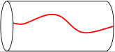
Gauge fixing of a twisted cylinder. (Note: the line is on the surface of the cylinder, not inside it.)

As an illustration of gauge fixing, one may look at a cylindrical rod and attempt to tell whether it is twisted. If the rod is perfectly cylindrical, then the circular symmetry of the cross section makes it impossible to tell whether or not it is twisted. However, if there were a straight line drawn along the length of the rod, then one could easily say whether or not there is a twist by looking at the state of the line. Drawing a line is gauge fixing. Drawing the line spoils the gauge symmetry, i.e., the circular symmetry U(1) of the cross section at each point of the rod. The line is the equivalent of a gauge function; it need not be straight. Almost any line is a valid gauge fixing, i.e., there is a large gauge freedom. In summary, to tell whether the rod is twisted, the gauge must be known. Physical quantities, such as the energy of the torsion, do not depend on the gauge, i.e., they are gauge invariant.

Coulomb gauge

The Coulomb gauge (also known as the transverse gauge) is used in quantum chemistry and condensed matter physics and is defined by the gauge condition (more precisely, gauge fixing condition)

$${\displaystyle \nabla \cdot {\mathbf {A} }(\mathbf {r} ,t)=0\,.}$$

It is particularly useful for "semi-classical" calculations in quantum mechanics, in which the vector potential is quantized but the Coulomb interaction is not.

The Coulomb gauge has a number of properties:

1. The potentials can be expressed in terms of instantaneous values of the fields and densities (in International System of Units) ^[1]
   $${\displaystyle \varphi (\mathbf {r} ,t)={\frac {1}{4\pi \varepsilon _{0}}}\int {\frac {\mathbf {\rho } (\mathbf {r} ',t)}{R}}d^{3}\mathbf {r} '}$$
   $${\displaystyle \mathbf {A} (\mathbf {r} ,t)=\nabla \times \int {\frac {\mathbf {B} (\mathbf {r} ',t)}{4\pi R}}d^{3}\mathbf {r} '}$$

   where ρ(r, t) is the electric charge density, ${\displaystyle \mathbf {R} =\mathbf {r} -\mathbf {r} '}$ and ${\displaystyle R=\left|\mathbf {R} \right|}$ (where r is any position vector in space and r′ is a point in the charge or current distribution), the ${\displaystyle \nabla }$ operates on r and d³ r is the volume element at r.

   The instantaneous nature of these potentials appears, at first sight, to violate causality, since motions of electric charge or magnetic field appear everywhere instantaneously as changes to the potentials. This is justified by noting that the scalar and vector potentials themselves do not affect the motions of charges, only the combinations of their derivatives that form the electromagnetic field strength. Although one can compute the field strengths explicitly in the Coulomb gauge and demonstrate that changes in them propagate at the speed of light, it is much simpler to observe that the field strengths are unchanged under gauge transformations and to demonstrate causality in the manifestly Lorentz covariant Lorenz gauge described below.

   Another expression for the vector potential, in terms of the time-retarded electric current density J(r, t), has been obtained to be: ^[2]

   $${\displaystyle \mathbf {A} (\mathbf {r} ,t)={\frac {1}{4\pi \varepsilon _{0}}}\,\nabla \times \int \left[\int _{0}^{R/c}\tau \,{\frac {{\mathbf {J} (\mathbf {r} ',t-\tau )}\times {\mathbf {R} }}{R^{3}}}\,d\tau \right]d^{3}\mathbf {r} '.}$$
2. Further gauge transformations that retain the Coulomb gauge condition might be made with gauge functions that satisfy ∇²ψ = 0, but as the only solution to this equation that vanishes at infinity (where all fields are required to vanish) is ψ(r, t) = 0, no gauge arbitrariness remains. Because of this, the Coulomb gauge is said to be a complete gauge, in contrast to gauges where some gauge arbitrariness remains, like the Lorenz gauge below.
3. The Coulomb gauge is a minimal gauge in the sense that the integral of A² over all space is minimal for this gauge: All other gauges give a larger integral. ^[3] The minimum value given by the Coulomb gauge is
   $${\displaystyle \int \mathbf {A} ^{2}(\mathbf {r} ,t)d^{3}\mathbf {r} =\iint {\frac {\mathbf {B} (\mathbf {r} ,t)\cdot \mathbf {B} (\mathbf {r} ',t)}{4\pi R}}d^{3}\mathbf {r} \,d^{3}\mathbf {r} '.}$$
4. In regions far from electric charge the scalar potential becomes zero. This is known as the radiation gauge. Electromagnetic radiation was first quantized in this gauge.
5. The Coulomb gauge admits a natural Hamiltonian formulation of the evolution equations of the electromagnetic field interacting with a conserved current,^{[ citation needed ]} which is an advantage for the quantization of the theory. The Coulomb gauge is, however, not Lorentz covariant. If a Lorentz transformation to a new inertial frame is carried out, a further gauge transformation has to be made to retain the Coulomb gauge condition. Because of this, the Coulomb gauge is not used in covariant perturbation theory, which has become standard for the treatment of relativistic quantum field theories such as quantum electrodynamics (QED). Lorentz covariant gauges such as the Lorenz gauge are usually used in these theories. Amplitudes of physical processes in QED in the noncovariant Coulomb gauge coincide with those in the covariant Lorenz gauge. ^[4]
6. For a uniform and constant magnetic field B the vector potential in the Coulomb gauge can be expressed in the so-called symmetric gauge as
   $${\displaystyle {\mathbf {A} }(\mathbf {r} ,t)=-{\frac {1}{2}}\mathbf {r} \times \mathbf {B} }$$

   plus the gradient of any scalar field (the gauge function), which can be confirmed by calculating the div and curl of A. The divergence of A at infinity is a consequence of the unphysical assumption that the magnetic field is uniform throughout the whole of space. Although this vector potential is unrealistic in general it can provide a good approximation to the potential in a finite volume of space in which the magnetic field is uniform. Another common choice for homogeneous constant fields is the Landau gauge (not to be confused with the R_ξ Landau gauge of the next section), where ${\displaystyle \mathbf {B} =B{\hat {z}}}$ and

   $${\displaystyle \mathbf {A} =B(\mathbf {r} \cdot {\hat {x}}){\hat {y}},}$$
   where ${\displaystyle {\hat {x}},{\hat {y}},{\hat {z}}}$ are unitary vectors of the Cartesian coordinate system (z-axis aligned with the magnetic field).
7. As a consequence of the considerations above, the electromagnetic potentials may be expressed in their most general forms in terms of the electromagnetic fields as
   $${\displaystyle \varphi (\mathbf {r} ,t)=\int {\frac {\nabla '\cdot {\mathbf {E} }(\mathbf {r} ',t)}{4\pi R}}\operatorname {d} \!^{3}\mathbf {r} '-{\frac {\partial {\psi (\mathbf {r} ,t)}}{\partial t}}}$$
   $${\displaystyle \mathbf {A} (\mathbf {r} ,t)=\nabla \times \int {\frac {\mathbf {B} (\mathbf {r} ',t)}{4\pi R}}\operatorname {d} \!^{3}\mathbf {r} '+\nabla \psi (\mathbf {r} ,t)}$$
   where ψ(r, t) is an arbitrary scalar field called the gauge function. The fields that are the derivatives of the gauge function are known as pure gauge fields and the arbitrariness associated with the gauge function is known as gauge freedom. In a calculation that is carried out correctly the pure gauge terms have no effect on any physical observable. A quantity or expression that does not depend on the gauge function is said to be gauge invariant: All physical observables are required to be gauge invariant. A gauge transformation from the Coulomb gauge to another gauge is made by taking the gauge function to be the sum of a specific function which will give the desired gauge transformation and the arbitrary function. If the arbitrary function is then set to zero, the gauge is said to be fixed. Calculations may be carried out in a fixed gauge but must be done in a way that is gauge invariant.

Lorenz gauge

Main article: Lorenz gauge condition

See also: Covariant formulation of classical electromagnetism

The Lorenz gauge is given, in SI units, by:

$${\displaystyle \nabla \cdot {\mathbf {A} }+{\frac {1}{c^{2}}}{\frac {\partial \varphi }{\partial t}}=0}$$

and in Gaussian units by:

$${\displaystyle \nabla \cdot {\mathbf {A} }+{\frac {1}{c}}{\frac {\partial \varphi }{\partial t}}=0.}$$

This may be rewritten as:

$${\displaystyle \partial _{\mu }A^{\mu }=0.}$$

where ${\displaystyle A^{\mu }=\left[\,{\tfrac {1}{c}}\varphi ,\,\mathbf {A} \,\right]}$ is the electromagnetic four-potential, ∂_μ the 4-gradient [using the metric signature (+, −, −, −)].

It is unique among the constraint gauges in retaining manifest Lorentz invariance. Note, however, that this gauge was originally named after the Danish physicist Ludvig Lorenz and not after Hendrik Lorentz; it is often misspelled "Lorentz gauge". (Neither was the first to use it in calculations; it was introduced in 1888 by George Francis FitzGerald.)

The Lorenz gauge leads to the following inhomogeneous wave equations for the potentials:

$${\displaystyle {\frac {1}{c^{2}}}{\frac {\partial ^{2}\varphi }{\partial t^{2}}}-\nabla ^{2}{\varphi }={\frac {\rho }{\varepsilon _{0}}}}$$

$${\displaystyle {\frac {1}{c^{2}}}{\frac {\partial ^{2}\mathbf {A} }{\partial t^{2}}}-\nabla ^{2}{\mathbf {A} }=\mu _{0}\mathbf {J} }$$

It can be seen from these equations that, in the absence of current and charge, the solutions are potentials which propagate at the speed of light.

The Lorenz gauge is incomplete in some sense: there remains a subspace of gauge transformations which can also preserve the constraint. These remaining degrees of freedom correspond to gauge functions which satisfy the wave equation

$${\displaystyle {\frac {\partial ^{2}\psi }{\partial t^{2}}}=c^{2}\nabla ^{2}\psi }$$

These remaining gauge degrees of freedom propagate at the speed of light. To obtain a fully fixed gauge, one must add boundary conditions along the light cone of the experimental region.

Maxwell's equations in the Lorenz gauge simplify to

$${\displaystyle \partial _{\mu }\partial ^{\mu }A^{\nu }=\mu _{0}j^{\nu }}$$

where ${\displaystyle j^{\nu }=\left[\,c\,\rho ,\,\mathbf {j} \,\right]}$ is the four-current.

Two solutions of these equations for the same current configuration differ by a solution of the vacuum wave equation

$${\displaystyle \partial _{\mu }\partial ^{\mu }A^{\nu }=0.}$$

In this form it is clear that the components of the potential separately satisfy the Klein–Gordon equation, and hence that the Lorenz gauge condition allows transversely, longitudinally, and "time-like" polarized waves in the four-potential. The transverse polarizations correspond to classical radiation, i.e., transversely polarized waves in the field strength. To suppress the "unphysical" longitudinal and time-like polarization states, which are not observed in experiments at classical distance scales, one must also employ auxiliary constraints known as Ward identities. Classically, these identities are equivalent to the continuity equation

$${\displaystyle \partial _{\mu }j^{\mu }=0.}$$

Many of the differences between classical and quantum electrodynamics can be accounted for by the role that the longitudinal and time-like polarizations play in interactions between charged particles at microscopic distances.

R_ξ gauges

The R_ξ gauges are a generalization of the Lorenz gauge applicable to theories expressed in terms of an action principle with Lagrangian density ${\displaystyle {\mathcal {L}}}$. Instead of fixing the gauge by constraining the gauge field a priori, via an auxiliary equation, one adds a gauge breaking term to the "physical" (gauge invariant) Lagrangian

$${\displaystyle \delta {\mathcal {L}}=-{\frac {\left(\partial _{\mu }A^{\mu }\right)^{2}}{2\xi }}}$$

The choice of the parameter ξ determines the choice of gauge. The R_ξ Landau gauge is classically equivalent to Lorenz gauge: it is obtained in the limit ξ → 0 but postpones taking that limit until after the theory has been quantized. It improves the rigor of certain existence and equivalence proofs. Most quantum field theory computations are simplest in the Feynman–'t Hooft gauge, in which ξ = 1; a few are more tractable in other R_ξ gauges, such as the Yennie gaugeξ = 3.

An equivalent formulation of R_ξ gauge uses an auxiliary field, a scalar field B with no independent dynamics:

$${\displaystyle \delta {\mathcal {L}}=B\,\partial _{\mu }A^{\mu }+{\frac {\xi }{2}}B^{2}}$$

The auxiliary field, sometimes called a Nakanishi–Lautrup field, can be eliminated by "completing the square" to obtain the previous form. From a mathematical perspective the auxiliary field is a variety of Goldstone boson, and its use has advantages when identifying the asymptotic states of the theory, and especially when generalizing beyond QED.

Historically, the use of R_ξ gauges was a significant technical advance in extending quantum electrodynamics computations beyond one-loop order. In addition to retaining manifest Lorentz invariance, the R_ξ prescription breaks the symmetry under local gauge transformations while preserving the ratio of functional measures of any two physically distinct gauge configurations. This permits a change of variables in which infinitesimal perturbations along "physical" directions in configuration space are entirely uncoupled from those along "unphysical" directions, allowing the latter to be absorbed into the physically meaningless normalization of the functional integral. When ξ is finite, each physical configuration (orbit of the group of gauge transformations) is represented not by a single solution of a constraint equation but by a Gaussian distribution centered on the extremum of the gauge breaking term. In terms of the Feynman rules of the gauge-fixed theory, this appears as a contribution to the photon propagator for internal lines from virtual photons of unphysical polarization.

The photon propagator, which is the multiplicative factor corresponding to an internal photon in the Feynman diagram expansion of a QED calculation, contains a factor g_μν corresponding to the Minkowski metric. An expansion of this factor as a sum over photon polarizations involves terms containing all four possible polarizations. Transversely polarized radiation can be expressed mathematically as a sum over either a linearly or circularly polarized basis. Similarly, one can combine the longitudinal and time-like gauge polarizations to obtain "forward" and "backward" polarizations; these are a form of light-cone coordinates in which the metric is off-diagonal. An expansion of the g_μν factor in terms of circularly polarized (spin ±1) and light-cone coordinates is called a spin sum. Spin sums can be very helpful both in simplifying expressions and in obtaining a physical understanding of the experimental effects associated with different terms in a theoretical calculation.

Richard Feynman used arguments along approximately these lines largely to justify calculation procedures that produced consistent, finite, high precision results for important observable parameters such as the anomalous magnetic moment of the electron. Although his arguments sometimes lacked mathematical rigor even by physicists' standards and glossed over details such as the derivation of Ward–Takahashi identities of the quantum theory, his calculations worked, and Freeman Dyson soon demonstrated that his method was substantially equivalent to those of Julian Schwinger and Sin-Itiro Tomonaga, with whom Feynman shared the 1965 Nobel Prize in Physics.

Forward and backward polarized radiation can be omitted in the asymptotic states of a quantum field theory (see Ward–Takahashi identity). For this reason, and because their appearance in spin sums can be seen as a mere mathematical device in QED (much like the electromagnetic four-potential in classical electrodynamics), they are often spoken of as "unphysical". But unlike the constraint-based gauge fixing procedures above, the R_ξ gauge generalizes well to non-abelian gauge groups such as the SU(3) of QCD. The couplings between physical and unphysical perturbation axes do not entirely disappear under the corresponding change of variables; to obtain correct results, one must account for the non-trivial Jacobian of the embedding of gauge freedom axes within the space of detailed configurations. This leads to the explicit appearance of forward and backward polarized gauge bosons in Feynman diagrams, along with Faddeev–Popov ghosts, which are even more "unphysical" in that they violate the spin–statistics theorem. The relationship between these entities, and the reasons why they do not appear as particles in the quantum mechanical sense, becomes more evident in the BRST formalism of quantization.

Maximal abelian gauge

In any non-abelian gauge theory, any maximal abelian gauge is an incomplete gauge which fixes the gauge freedom outside of the maximal abelian subgroup. Examples are

• For SU(2) gauge theory in D dimensions, the maximal abelian subgroup is a U(1) subgroup. If this is chosen to be the one generated by the Pauli matrix σ₃, then the maximal abelian gauge is that which maximizes the function
  $${\displaystyle \int d^{D}x\left[\left(A_{\mu }^{1}\right)^{2}+\left(A_{\mu }^{2}\right)^{2}\right]\,,}$$
  where
  $${\displaystyle {\mathbf {A} }_{\mu }=A_{\mu }^{a}\sigma _{a}\,.}$$
• For SU(3) gauge theory in D dimensions, the maximal abelian subgroup is a U(1)×U(1) subgroup. If this is chosen to be the one generated by the Gell-Mann matrices λ₃ and λ₈, then the maximal abelian gauge is that which maximizes the function
  $${\displaystyle \int d^{D}x\left[\left(A_{\mu }^{1}\right)^{2}+\left(A_{\mu }^{2}\right)^{2}+\left(A_{\mu }^{4}\right)^{2}+\left(A_{\mu }^{5}\right)^{2}+\left(A_{\mu }^{6}\right)^{2}+\left(A_{\mu }^{7}\right)^{2}\right]\,,}$$
  where
  $${\displaystyle {\mathbf {A} }_{\mu }=A_{\mu }^{a}\lambda _{a}}$$

This applies regularly in higher algebras (of groups in the algebras), for example the Clifford Algebra and as it is regularly.

Less commonly used gauges

Various other gauges, which can be beneficial in specific situations have appeared in the literature. ^[2]

Weyl gauge

The Weyl gauge (also known as the Hamiltonian or temporal gauge) is an incomplete gauge obtained by the choice

$${\displaystyle \varphi =0}$$

It is named after Hermann Weyl. It eliminates the negative-norm ghost, lacks manifest Lorentz invariance, and requires longitudinal photons and a constraint on states. ^[5]

Multipolar gauge

The gauge condition of the multipolar gauge (also known as the line gauge, point gauge or Poincaré gauge (named after Henri Poincaré)) is:

$${\displaystyle \mathbf {r} \cdot \mathbf {A} =0.}$$

This is another gauge in which the potentials can be expressed in a simple way in terms of the instantaneous fields

$${\displaystyle \mathbf {A} (\mathbf {r} ,t)=-\mathbf {r} \times \int _{0}^{1}\mathbf {B} (u\mathbf {r} ,t)u\,du}$$

$${\displaystyle \varphi (\mathbf {r} ,t)=-\mathbf {r} \cdot \int _{0}^{1}\mathbf {E} (u\mathbf {r} ,t)du.}$$

Fock–Schwinger gauge

The gauge condition of the Fock–Schwinger gauge (named after Vladimir Fock and Julian Schwinger; sometimes also called the relativistic Poincaré gauge) is:

$${\displaystyle x^{\mu }A_{\mu }=0}$$

where x^μ is the position four-vector.

Dirac gauge

The nonlinear Dirac gauge condition (named after Paul Dirac) is:

$${\displaystyle A_{\mu }A^{\mu }=k^{2}}$$

References

1. Stewart, A. M. (2003). "Vector potential of the Coulomb gauge". European Journal of Physics . 24 (5): 519–524. Bibcode:2003EJPh...24..519S. doi:10.1088/0143-0807/24/5/308. S2CID   250880504.
2. Jackson, J. D. (2002). "From Lorenz to Coulomb and other explicit gauge transformations". American Journal of Physics . 70 (9): 917–928. arXiv: physics/0204034 . Bibcode:2002AmJPh..70..917J. doi:10.1119/1.1491265. S2CID   119652556.
3. Gubarev, F. V.; Stodolsky, L.; Zakharov, V. I. (2001). "On the Significance of the Vector Potential Squared". Phys. Rev. Lett. 86 (11): 2220–2222. arXiv: hep-ph/0010057 . Bibcode:2001PhRvL..86.2220G. doi:10.1103/PhysRevLett.86.2220. PMID   11289894. S2CID   45172403.
4. Adkins, Gregory S. (1987-09-15). "Feynman rules of Coulomb-gauge QED and the electron magnetic moment". Physical Review D. 36 (6). American Physical Society (APS): 1929–1932. Bibcode:1987PhRvD..36.1929A. doi:10.1103/physrevd.36.1929. ISSN   0556-2821. PMID   9958379.
5. Hatfield, Brian (1992). Quantum field theory of point particles and strings. Addison-Wesley. pp. 210–213. ISBN   0201360799.

Further reading

• Landau, Lev; Lifshitz, Evgeny (2007). The classical theory of fields. Amsterdam: Elsevier Butterworth Heinemann. ISBN   978-0-7506-2768-9.
• Jackson, J. D. (1999). Classical Electrodynamics (3rd ed.). New York: Wiley. ISBN   0-471-30932-X.