Thermal wind

Last updated
Jet streams (shown in pink) are well-known examples of thermal wind. They arise from the horizontal temperature gradients between the warm tropics and the colder polar regions. Jet stream.jpg
Jet streams (shown in pink) are well-known examples of thermal wind. They arise from the horizontal temperature gradients between the warm tropics and the colder polar regions.

In atmospheric science, the thermal wind is the vector difference between the geostrophic wind at upper altitudes minus that at lower altitudes in the atmosphere. It is the hypothetical vertical wind shear that would exist if the winds obey geostrophic balance in the horizontal, while pressure obeys hydrostatic balance in the vertical. The combination of these two force balances is called thermal wind balance, a term generalizable also to more complicated horizontal flow balances such as gradient wind balance.

Contents

Since the geostrophic wind at a given pressure level flows along geopotential height contours on a map, and the geopotential thickness of a pressure layer is proportional to virtual temperature, it follows that the thermal wind flows along thickness or temperature contours. For instance, the thermal wind associated with pole-to-equator temperature gradients is the primary physical explanation for the jet stream in the upper half of the troposphere, which is the atmospheric layer extending from the surface of the planet up to altitudes of about 12–15 km.

Mathematically, the thermal wind relation defines a vertical wind shear – a variation in wind speed or direction with height. The wind shear in this case is a function of a horizontal temperature gradient, which is a variation in temperature over some horizontal distance. Also called baroclinic flow, the thermal wind varies with height in proportion to the horizontal temperature gradient. The thermal wind relation results from hydrostatic balance and geostrophic balance in the presence of a temperature gradient along constant pressure surfaces, or isobars.

The term thermal wind is often considered a misnomer, since it really describes the change in wind with height, rather than the wind itself. However, one can view the thermal wind as a geostrophic wind that varies with height, so that the term wind seems appropriate. In the early years of meteorology, when data was scarce, the wind field could be estimated using the thermal wind relation and knowledge of a surface wind speed and direction as well as thermodynamic soundings aloft. [1] In this way, the thermal wind relation acts to define the wind itself, rather than just its shear. Many authors retain the thermal wind moniker, even though it describes a wind gradient, sometimes offering a clarification to that effect.

Description

Physical explanation

The thermal wind is the change in the amplitude or sign of the geostrophic wind due to a horizontal temperature gradient. The geostrophic wind is an idealized wind that results from a balance of forces along a horizontal dimension. Whenever the Earth's rotation plays a dominant role in fluid dynamics, as in the mid-latitudes, a balance between the Coriolis force and the pressure-gradient force develops. Intuitively, a horizontal difference in pressure pushes air across that difference in a similar way that the horizontal difference in the height of a hill causes objects to roll downhill. However, the Coriolis force intervenes and nudges the air towards the right (in the northern hemisphere). This is illustrated in panel (a) of the figure below. The balance that develops between these two forces results in a flow that parallels the horizontal pressure difference, or pressure gradient. [1] In addition, when forces acting in the vertical dimension are dominated by the vertical pressure-gradient force and the gravitational force, hydrostatic balance occurs.

The geostrophic wind on different isobaric levels in a barotropic atmosphere (a) and in a baroclinic atmosphere (b). The blue portion of the surface denotes a cold region while the orange portion denotes a warm region. This temperature structure is restricted to the surface in (a) but extends through the depth of the fluid in (b). The dotted lines enclose isobaric surfaces which remain at constant slope with increasing height in (a) and increase in slope with height in (b). Pink arrows illustrate the direction and amplitude of the horizontal wind. Only in the baroclinic atmosphere (b) do these vary with height. Such variation illustrates the thermal wind. Thermal wind, Baroclinic & Barotropic Atmospheres.jpg
The geostrophic wind on different isobaric levels in a barotropic atmosphere (a) and in a baroclinic atmosphere (b). The blue portion of the surface denotes a cold region while the orange portion denotes a warm region. This temperature structure is restricted to the surface in (a) but extends through the depth of the fluid in (b). The dotted lines enclose isobaric surfaces which remain at constant slope with increasing height in (a) and increase in slope with height in (b). Pink arrows illustrate the direction and amplitude of the horizontal wind. Only in the baroclinic atmosphere (b) do these vary with height. Such variation illustrates the thermal wind.

In a barotropic atmosphere, where density is a function only of pressure, a horizontal pressure gradient will drive a geostrophic wind that is constant with height. However, if a horizontal temperature gradient exists along isobars, the isobars will also vary with the temperature. In the mid-latitudes there often is a positive coupling between pressure and temperature. Such a coupling causes the slope of the isobars to increase with height, as illustrated in panel (b) of the figure to the left. Because isobars are steeper at higher elevations, the associated pressure gradient force is stronger there. However, the Coriolis force is the same, so the resulting geostrophic wind at higher elevations must be greater in the direction of the pressure force. [2]

In a baroclinic atmosphere, where density is a function of both pressure and temperature, such horizontal temperature gradients can exist. The difference in horizontal wind speed with height that results is a vertical wind shear, traditionally called the thermal wind. [2]

Mathematical formalism

The geopotential thickness of an atmospheric layer defined by two different pressures is described by the hypsometric equation:

,

where is the specific gas constant for air, is the geopotential at pressure level , and is the vertically-averaged temperature of the layer. This formula shows that the layer thickness is proportional to the temperature. When there is a horizontal temperature gradient, the thickness of the layer would be greatest where the temperature is greatest.

Differentiating the geostrophic wind, (where is the Coriolis parameter, is the vertical unit vector, and the subscript "p" on the gradient operator denotes gradient on a constant pressure surface) with respect to pressure, and integrate from pressure level to , we obtain the thermal wind equation:

.

Substituting the hypsometric equation, one gets a form based on temperature,

.

Note that thermal wind is at right angles to the horizontal temperature gradient, counter clockwise in the northern hemisphere. In the southern hemisphere, the change in sign of flips the direction.

Examples

Advection turning

In (a), cold advection is occurring, so the thermal wind causes the geostrophic wind to rotate counterclockwise (for the northern hemisphere) with height. In (b), warm advection is occurring, so the geostrophic wind rotates clockwise with height. Backing and veering.jpg
In (a), cold advection is occurring, so the thermal wind causes the geostrophic wind to rotate counterclockwise (for the northern hemisphere) with height. In (b), warm advection is occurring, so the geostrophic wind rotates clockwise with height.

If a component of the geostrophic wind is parallel to the temperature gradient, the thermal wind will cause the geostrophic wind to rotate with height. If geostrophic wind blows from cold air to warm air (cold advection) the geostrophic wind will turn counterclockwise with height (for the northern hemisphere), a phenomenon known as wind backing. Otherwise, if geostrophic wind blows from warm air to cold air (warm advection) the wind will turn clockwise with height, also known as wind veering.

Wind backing and veering allow an estimation of the horizontal temperature gradient with data from an atmospheric sounding.

Frontogenesis

As in the case of advection turning, when there is a cross-isothermal component of the geostrophic wind, a sharpening of the temperature gradient results. Thermal wind causes a deformation field and frontogenesis may occur.

Jet stream

A horizontal temperature gradient exists while moving North-South along a meridian because curvature of the Earth allows for more solar heating at the equator than at the poles. This creates a westerly geostrophic wind pattern to form in the mid-latitudes. Because thermal wind causes an increase in wind velocity with height, the westerly pattern increases in intensity up until the tropopause, creating a strong wind current known as the jet stream. The Northern and Southern Hemispheres exhibit similar jet stream patterns in the mid-latitudes.

The strongest part of jet streams should be in proximity where temperature gradients are the largest. Due to land masses in the northern hemisphere, largest temperature contrasts are observed on the east coast of North America (boundary between Canadian cold air mass and the Gulf Stream/warmer Atlantic) and Eurasia (boundary between the boreal winter monsoon/Siberian cold air mass and the warm Pacific). Therefore, the strongest boreal winter jet streams are observed over east coast of North America and Eurasia. Since stronger vertical shear promotes baroclinic instability, the most rapid development of extratropical cyclones (so called bombs) is also observed along the east coast of North America and Eurasia.

The lack of land masses in the Southern Hemisphere leads to a more constant jet with longitude (i.e. a more zonally symmetric jet).

Related Research Articles

Geopotential height or geopotential altitude is a vertical coordinate referenced to Earth's mean sea level that represents the work done by lifting one unit mass one unit distance through a region in which the acceleration of gravity is uniformly 9.80665 m/s2. Geopotential height (altitude) differs from geometric (tapeline) height but remains a historical convention in aeronautics as the altitude used for calibration of aircraft barometric altimeters.

The barotropic vorticity equation assumes the atmosphere is nearly barotropic, which means that the direction and speed of the geostrophic wind are independent of height. In other words, there is no vertical wind shear of the geostrophic wind. It also implies that thickness contours are parallel to upper level height contours. In this type of atmosphere, high and low pressure areas are centers of warm and cold temperature anomalies. Warm-core highs and cold-core lows have strengthening winds with height, with the reverse true for cold-core highs and warm-core lows.

Geopotential is the potential of the Earth's gravity field. For convenience it is often defined as the negative of the potential energy per unit mass, so that the gravity vector is obtained as the gradient of the geopotential, without the negation. In addition to the actual potential, a hypothetical normal potential and their difference, the disturbing potential, can also be defined.

<span class="mw-page-title-main">Wind shear</span> Difference in wind speed or direction over a short distance

Wind shear, sometimes referred to as wind gradient, is a difference in wind speed and/or direction over a relatively short distance in the atmosphere. Atmospheric wind shear is normally described as either vertical or horizontal wind shear. Vertical wind shear is a change in wind speed or direction with a change in altitude. Horizontal wind shear is a change in wind speed with a change in lateral position for a given altitude.

The primitive equations are a set of nonlinear partial differential equations that are used to approximate global atmospheric flow and are used in most atmospheric models. They consist of three main sets of balance equations:

  1. A continuity equation: Representing the conservation of mass.
  2. Conservation of momentum: Consisting of a form of the Navier–Stokes equations that describe hydrodynamical flow on the surface of a sphere under the assumption that vertical motion is much smaller than horizontal motion (hydrostasis) and that the fluid layer depth is small compared to the radius of the sphere
  3. A thermal energy equation: Relating the overall temperature of the system to heat sources and sinks

In atmospheric science, geostrophic flow is the theoretical wind that would result from an exact balance between the Coriolis force and the pressure gradient force. This condition is called geostrophic equilibrium or geostrophic balance. The geostrophic wind is directed parallel to isobars. This balance seldom holds exactly in nature. The true wind almost always differs from the geostrophic wind due to other forces such as friction from the ground. Thus, the actual wind would equal the geostrophic wind only if there were no friction and the isobars were perfectly straight. Despite this, much of the atmosphere outside the tropics is close to geostrophic flow much of the time and it is a valuable first approximation. Geostrophic flow in air or water is a zero-frequency inertial wave.

<span class="mw-page-title-main">Planetary boundary layer</span> Lowest part of the atmosphere directly influenced by contact with the planetary surface

In meteorology, the planetary boundary layer (PBL), also known as the atmospheric boundary layer (ABL) or peplosphere, is the lowest part of the atmosphere and its behaviour is directly influenced by its contact with a planetary surface. On Earth it usually responds to changes in surface radiative forcing in an hour or less. In this layer physical quantities such as flow velocity, temperature, and moisture display rapid fluctuations (turbulence) and vertical mixing is strong. Above the PBL is the "free atmosphere", where the wind is approximately geostrophic, while within the PBL the wind is affected by surface drag and turns across the isobars.

The oceanic, wind driven Ekman spiral is the result of a force balance created by a shear stress force, Coriolis force and the water drag. This force balance gives a resulting current of the water different from the winds. In the ocean, there are two places where the Ekman spiral can be observed. At the surface of the ocean, the shear stress force corresponds with the wind stress force. At the bottom of the ocean, the shear stress force is created by friction with the ocean floor. This phenomenon was first observed at the surface by the Norwegian oceanographer Fridtjof Nansen during his Fram expedition. He noticed that icebergs did not drift in the same direction as the wind. His student, the Swedish oceanographer Vagn Walfrid Ekman, was the first person to physically explain this process.

In meteorology, air currents are concentrated areas of winds. They are mainly due to differences in atmospheric pressure or temperature. They are divided into horizontal and vertical currents; both are present at mesoscale while horizontal ones dominate at synoptic scale. Air currents are not only found in the troposphere, but extend to the stratosphere and mesosphere.

In atmospheric science, the pressure gradient is a physical quantity that describes in which direction and at what rate the pressure increases the most rapidly around a particular location. The pressure gradient is a dimensional quantity expressed in units of pascals per metre (Pa/m). Mathematically, it is the gradient of pressure as a function of position. The negative gradient of pressure is known as the force density.

In fluid mechanics, potential vorticity (PV) is a quantity which is proportional to the dot product of vorticity and stratification. This quantity, following a parcel of air or water, can only be changed by adiabatic or frictional processes. It is a useful concept for understanding the generation of vorticity in cyclogenesis, especially along the polar front, and in analyzing flow in the ocean.

<span class="mw-page-title-main">Geostrophic current</span> Oceanic flow in which the pressure gradient force is balanced by the Coriolis effect

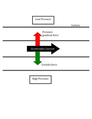
A geostrophic current is an oceanic current in which the pressure gradient force is balanced by the Coriolis effect. The direction of geostrophic flow is parallel to the isobars, with the high pressure to the right of the flow in the Northern Hemisphere, and the high pressure to the left in the Southern Hemisphere. This concept is familiar from weather maps, whose isobars show the direction of geostrophic winds. Geostrophic flow may be either barotropic or baroclinic. A geostrophic current may also be thought of as a rotating shallow water wave with a frequency of zero.

Frontogenesis is a meteorological process of tightening of horizontal temperature gradients to produce fronts. In the end, two types of fronts form: cold fronts and warm fronts. A cold front is a narrow line where temperature decreases rapidly. A warm front is a narrow line of warmer temperatures and essentially where much of the precipitation occurs. Frontogenesis occurs as a result of a developing baroclinic wave. According to Hoskins & Bretherton, there are eight mechanisms that influence temperature gradients: horizontal deformation, horizontal shearing, vertical deformation, differential vertical motion, latent heat release, surface friction, turbulence and mixing, and radiation. Semigeostrophic frontogenesis theory focuses on the role of horizontal deformation and shear.

In atmospheric science, balanced flow is an idealisation of atmospheric motion. The idealisation consists in considering the behaviour of one isolated parcel of air having constant density, its motion on a horizontal plane subject to selected forces acting on it and, finally, steady-state conditions.

The omega equation is a culminating result in synoptic-scale meteorology. It is an elliptic partial differential equation, named because its left-hand side produces an estimate of vertical velocity, customarily expressed by symbol , in a pressure coordinate measuring height the atmosphere. Mathematically, , where represents a material derivative. The underlying concept is more general, however, and can also be applied to the Boussinesq fluid equation system where vertical velocity is in altitude coordinate z.

In oceanography, Ekman velocity – also referred as a kind of the residual ageostrophic velocity as it deviates from geostrophy – is part of the total horizontal velocity (u) in the upper layer of water of the open ocean. This velocity, caused by winds blowing over the surface of the ocean, is such that the Coriolis force on this layer is balanced by the force of the wind.

Q-vectors are used in atmospheric dynamics to understand physical processes such as vertical motion and frontogenesis. Q-vectors are not physical quantities that can be measured in the atmosphere but are derived from the quasi-geostrophic equations and can be used in the previous diagnostic situations. On meteorological charts, Q-vectors point toward upward motion and away from downward motion. Q-vectors are an alternative to the omega equation for diagnosing vertical motion in the quasi-geostrophic equations.

While geostrophic motion refers to the wind that would result from an exact balance between the Coriolis force and horizontal pressure-gradient forces, quasi-geostrophic (QG) motion refers to flows where the Coriolis force and pressure gradient forces are almost in balance, but with inertia also having an effect.

A baroclinic instability is a fluid dynamical instability of fundamental importance in the atmosphere and ocean. It can lead to the formation of transient mesoscale eddies, with a horizontal scale of 10-100 km. In contrast, flows on the largest scale in the ocean are described as ocean currents, the largest scale eddies are mostly created by shearing of two ocean currents and static mesoscale eddies are formed by the flow around an obstacle (as seen in the animation on eddy. Mesoscale eddies are circular currents with swirling motion and account for approximately 90% of the ocean's total kinetic energy. Therefore, they are key in mixing and transport of for example heat, salt and nutrients.

Atmospheric circulation of a planet is largely specific to the planet in question and the study of atmospheric circulation of exoplanets is a nascent field as direct observations of exoplanet atmospheres are still quite sparse. However, by considering the fundamental principles of fluid dynamics and imposing various limiting assumptions, a theoretical understanding of atmospheric motions can be developed. This theoretical framework can also be applied to planets within the Solar System and compared against direct observations of these planets, which have been studied more extensively than exoplanets, to validate the theory and understand its limitations as well.

References

  1. 1 2 Cushman-Roisin, Benoit (1994). Introduction to Geophysical Fluid Dynamics. Prentice-Hall, Inc. ISBN   0-13-353301-8.
  2. 1 2 Holton, James (2004). An Introduction to Dynamic Meteorology. Elsevier.

Further reading