
Climate is the long-term weather pattern in a region, typically averaged over 30 years. More rigorously, it is the mean and variability of meteorological variables over a time spanning from months to millions of years. Some of the meteorological variables that are commonly measured are temperature, humidity, atmospheric pressure, wind, and precipitation. In a broader sense, climate is the state of the components of the climate system, including the atmosphere, hydrosphere, cryosphere, lithosphere and biosphere and the interactions between them. The climate of a location is affected by its latitude, longitude, terrain, altitude, land use and nearby water bodies and their currents.

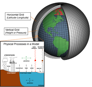
Numerical climate models are mathematical models that can simulate the interactions of important drivers of climate. These drivers are the atmosphere, oceans, land surface and ice. Scientists use climate models to study the dynamics of the climate system and to make projections of future climate and of climate change. Climate models can also be qualitative models and contain narratives, largely descriptive, of possible futures.

Climatology or climate science is the scientific study of Earth's climate, typically defined as weather conditions averaged over a period of at least 30 years. Climate concerns the atmospheric condition during an extended to indefinite period of time; weather is the condition of the atmosphere during a relative brief period of time. The main topics of research are the study of climate variability, mechanisms of climate changes and modern climate change. This topic of study is regarded as part of the atmospheric sciences and a subdivision of physical geography, which is one of the Earth sciences. Climatology includes some aspects of oceanography and biogeochemistry.
A general circulation model (GCM) is a type of climate model. It employs a mathematical model of the general circulation of a planetary atmosphere or ocean. It uses the Navier–Stokes equations on a rotating sphere with thermodynamic terms for various energy sources. These equations are the basis for computer programs used to simulate the Earth's atmosphere or oceans. Atmospheric and oceanic GCMs are key components along with sea ice and land-surface components.
Numerical weather prediction (NWP) uses mathematical models of the atmosphere and oceans to predict the weather based on current weather conditions. Though first attempted in the 1920s, it was not until the advent of computer simulation in the 1950s that numerical weather predictions produced realistic results. A number of global and regional forecast models are run in different countries worldwide, using current weather observations relayed from radiosondes, weather satellites and other observing systems as inputs.
In climatology, the Coupled Model Intercomparison Project (CMIP) is a collaborative framework designed to improve knowledge of climate change. It was organized in 1995 by the Working Group on Coupled Modelling (WGCM) of the World Climate Research Programme (WCRP). It is developed in phases to foster the climate model improvements but also to support national and international assessments of climate change. A related project is the Atmospheric Model Intercomparison Project (AMIP) for global coupled ocean-atmosphere general circulation models (GCMs).

Ensemble forecasting is a method used in or within numerical weather prediction. Instead of making a single forecast of the most likely weather, a set of forecasts is produced. This set of forecasts aims to give an indication of the range of possible future states of the atmosphere.
Data assimilation refers to a large group of methods that update information from numerical computer models with information from observations. Data assimilation is used to update model states, model trajectories over time, model parameters, and combinations thereof. What distinguishes data assimilation from other estimation methods is that the computer model is a dynamical model, i.e. the model describes how model variables change over time, and its firm mathematical foundation in Bayesian Inference. As such, it generalizes inverse methods and has close connections with machine learning.

Spatial analysis is any of the formal techniques which studies entities using their topological, geometric, or geographic properties. Spatial analysis includes a variety of techniques using different analytic approaches, especially spatial statistics. It may be applied in fields as diverse as astronomy, with its studies of the placement of galaxies in the cosmos, or to chip fabrication engineering, with its use of "place and route" algorithms to build complex wiring structures. In a more restricted sense, spatial analysis is geospatial analysis, the technique applied to structures at the human scale, most notably in the analysis of geographic data. It may also be applied to genomics, as in transcriptomics data.

In atmospheric science, an atmospheric model is a mathematical model constructed around the full set of primitive, dynamical equations which govern atmospheric motions. It can supplement these equations with parameterizations for turbulent diffusion, radiation, moist processes, heat exchange, soil, vegetation, surface water, the kinematic effects of terrain, and convection. Most atmospheric models are numerical, i.e. they discretize equations of motion. They can predict microscale phenomena such as tornadoes and boundary layer eddies, sub-microscale turbulent flow over buildings, as well as synoptic and global flows. The horizontal domain of a model is either global, covering the entire Earth, or regional (limited-area), covering only part of the Earth. Atmospheric models also differ in how they compute vertical fluid motions; some types of models are thermotropic, barotropic, hydrostatic, and non-hydrostatic. These model types are differentiated by their assumptions about the atmosphere, which must balance computational speed with the model's fidelity to the atmosphere it is simulating.
Geophysical Fluid Dynamics Laboratory Coupled Model is a coupled atmosphere–ocean general circulation model (AOGCM) developed at the NOAA Geophysical Fluid Dynamics Laboratory in the United States. It is one of the leading climate models used in the Fourth Assessment Report of the IPCC, along with models developed at the Max Planck Institute for Climate Research, the Hadley Centre and the National Center for Atmospheric Research.
Tom Michael Lampe Wigley is a climate scientist at the University of Adelaide. He is also affiliated with the University Corporation for Atmospheric Research. He was named a fellow of the American Association for the Advancement of Science (AAAS) for his major contributions to climate and carbon cycle modeling and to climate data analysis, and because he is "one of the world's foremost experts on climate change and one of the most highly cited scientists in the discipline." His Web of Science h-index is 75, and his Google Scholar h-index is 114. He has contributed to many of the reports published by the Intergovernmental Panel on Climate Change (IPCC), a body that was recognized in 2007 by the joint award of the 2007 Nobel Peace Prize.
An atmospheric reanalysis is a meteorological and climate data assimilation project which aims to assimilate historical atmospheric observational data spanning an extended period, using a single consistent assimilation scheme throughout.
RheinBlick2050 is an environmental science research project on the impacts of regional climate change on discharge of the Rhine River and its major tributaries in Central Europe. The project runtime was from January 2008 until September 2010, initiated by and coordinated on behalf of the International Commission for the Hydrology of the Rhine Basin (CHR).
Ocean general circulation models (OGCMs) are a particular kind of general circulation model to describe physical and thermodynamical processes in oceans. The oceanic general circulation is defined as the horizontal space scale and time scale larger than mesoscale. They depict oceans using a three-dimensional grid that include active thermodynamics and hence are most directly applicable to climate studies. They are the most advanced tools currently available for simulating the response of the global ocean system to increasing greenhouse gas concentrations. A hierarchy of OGCMs have been developed that include varying degrees of spatial coverage, resolution, geographical realism, process detail, etc.
The field of complex networks has emerged as an important area of science to generate novel insights into nature of complex systems The application of network theory to climate science is a young and emerging field. To identify and analyze patterns in global climate, scientists model climate data as complex networks.
Earth systems models of intermediate complexity (EMICs) form an important class of climate models, primarily used to investigate the earth's systems on long timescales or at reduced computational cost. This is mostly achieved through operation at lower temporal and spatial resolution than more comprehensive general circulation models (GCMs). Due to the nonlinear relationship between spatial resolution and model run-speed, modest reductions in resolution can lead to large improvements in model run-speed. This has historically allowed the inclusion of previously unincorporated earth-systems such as ice sheets and carbon cycle feedbacks. These benefits are conventionally understood to come at the cost of some model accuracy. However, the degree to which higher resolution models improve accuracy rather than simply precision is contested.
The Fisheries and Marine Ecosystem Model Intercomparison Project (Fish-MIP) is a marine biology project to compare computer models of the impact of climate change on sea life. Founded in 2013 as part of the Inter-Sectoral Impact Model Intercomparison Project (ISIMIP), it was established to answer questions about the future of marine biodiversity, seafood supply, fisheries, and marine ecosystem functioning in the context of various climate change scenarios. It combines diverse marine ecosystem models from both the global and regional scale through a standardized protocol for ensemble modelling in an attempt to correct for any bias in the individual models that make up the ensemble. Fish-MIP's goal is to use this ensemble modelling to project a more robust picture of the future state of fisheries and marine ecosystems under the impacts of climate change, and ultimately to help inform fishing policy.
Boualem Khouider is an Algerian-Canadian applied mathematician, climate scientist, academic, and author. He is a professor, and former Chair of Mathematics and Statistics at the University of Victoria.
Volker Wulfmeyer is a German physicist, meteorologist, climate and earth system researcher, university professor, and member of the Heidelberg Academy of Sciences.