Remote sensing

Not to be confused with remote viewing.

For other uses, see Remote sensing (disambiguation).

Synthetic aperture radar image of Death Valley colored using polarimetry

Remote sensing is the acquisition of information about an object or phenomenon without making physical contact with the object, in contrast to in situ or on-site observation. The term is applied especially to acquiring information about Earth and other planets. Remote sensing is used in numerous fields, including geophysics, geography, land surveying and most Earth science disciplines (e.g. exploration geophysics, hydrology, ecology, meteorology, oceanography, glaciology, geology). It also has military, intelligence, commercial, economic, planning, and humanitarian applications, among others.

In current usage, the term remote sensing generally refers to the use of satellite- or aircraft-based sensor technologies to detect and classify objects on Earth. It includes the surface and the atmosphere and oceans, based on propagated signals (e.g. electromagnetic radiation). It may be split into "active" remote sensing (when a signal is emitted by a satellite or aircraft to the object and its reflection is detected by the sensor) and "passive" remote sensing (when the reflection of sunlight is detected by the sensor). ^{[1] [2] [3] [4]}

Overview

This video is about how Landsat was used to identify areas of conservation in the Democratic Republic of the Congo, and how it was used to help map an area called MLW in the north.

Remote sensing can be divided into two types of methods: Passive remote sensing and Active remote sensing. Passive sensors gather radiation that is emitted or reflected by the object or surrounding areas. Reflected sunlight is the most common source of radiation measured by passive sensors. Examples of passive remote sensors include film photography, infrared, charge-coupled devices, and radiometers. Active collection, on the other hand, emits energy in order to scan objects and areas whereupon a sensor then detects and measures the radiation that is reflected or backscattered from the target. RADAR and LiDAR are examples of active remote sensing where the time delay between emission and return is measured, establishing the location, speed and direction of an object.

Illustration of remote sensing

Remote sensing makes it possible to collect data of dangerous or inaccessible areas. Remote sensing applications include monitoring deforestation in areas such as the Amazon Basin, glacial features in Arctic and Antarctic regions, and depth sounding of coastal and ocean depths. Military collection during the Cold War made use of stand-off collection of data about dangerous border areas. Remote sensing also replaces costly and slow data collection on the ground, ensuring in the process that areas or objects are not disturbed.

Orbital platforms collect and transmit data from different parts of the electromagnetic spectrum, which in conjunction with larger scale aerial or ground-based sensing and analysis, provides researchers with enough information to monitor trends such as El Niño and other natural long and short term phenomena. Other uses include different areas of the earth sciences such as natural resource management, agricultural fields such as land usage and conservation, ^{[5] [6]} greenhouse gas monitoring, ^[7] oil spill detection and monitoring, ^[8] and national security and overhead, ground-based and stand-off collection on border areas. ^[9]

Types of data acquisition techniques

The basis for multispectral collection and analysis is that of examined areas or objects that reflect or emit radiation that stand out from surrounding areas. For a summary of major remote sensing satellite systems see the overview table.

Applications of remote sensing

Further information: Remote sensing (geology) and Remote sensing in archaeology

Radar image of Aswan Dam, Egypt taken by Umbra

• Conventional radar is mostly associated with aerial traffic control, early warning, and certain large-scale meteorological data. Doppler radar is used by local law enforcements' monitoring of speed limits and in enhanced meteorological collection such as wind speed and direction within weather systems in addition to precipitation location and intensity. Other types of active collection includes plasmas in the ionosphere. Interferometric synthetic aperture radar is used to produce precise digital elevation models of large scale terrain (See RADARSAT, TerraSAR-X, Magellan).
• Laser and radar altimeters on satellites have provided a wide range of data. By measuring the bulges of water caused by gravity, they map features on the seafloor to a resolution of a mile or so. By measuring the height and wavelength of ocean waves, the altimeters measure wind speeds and direction, and surface ocean currents and directions.
• Ultrasound (acoustic) and radar tide gauges measure sea level, tides and wave direction in coastal and offshore tide gauges.
• Light detection and ranging (LIDAR) is well known in examples of weapon ranging, laser illuminated homing of projectiles. LIDAR is used to detect and measure the concentration of various chemicals in the atmosphere, while airborne LIDAR can be used to measure the heights of objects and features on the ground more accurately than with radar technology. Vegetation remote sensing is a principal application of LIDAR. ^[10]
• Radiometers and photometers are the most common instrument in use, collecting reflected and emitted radiation in a wide range of frequencies. The most common are visible and infrared sensors, followed by microwave, gamma-ray, and rarely, ultraviolet. They may also be used to detect the emission spectra of various chemicals, providing data on chemical concentrations in the atmosphere.

Examples of remote sensing equipment deployed by
or interfaced with oceanographic research vessels.

• Radiometers are also used at night, because artificial light emissions are a key signature of human activity. ^[12] Applications include remote sensing of population, GDP, and damage to infrastructure from war or disasters.
• Radiometers and radar onboard of satellites can be used to monitor volcanic eruptions ^{[13] [14]}
• Spectropolarimetric Imaging has been reported to be useful for target tracking purposes by researchers at the U.S. Army Research Laboratory. They determined that manmade items possess polarimetric signatures that are not found in natural objects. These conclusions were drawn from the imaging of military trucks, like the Humvee, and trailers with their acousto-optic tunable filter dual hyperspectral and spectropolarimetric VNIR Spectropolarimetric Imager. ^{[15] [16]}
• Stereographic pairs of aerial photographs have often been used to make topographic maps by imagery and terrain analysts in trafficability and highway departments for potential routes, in addition to modelling terrestrial habitat features. ^{[17] [18] [19]}
• Simultaneous multi-spectral platforms such as Landsat have been in use since the 1970s. These thematic mappers take images in multiple wavelengths of electromagnetic radiation (multi-spectral) and are usually found on Earth observation satellites, including (for example) the Landsat program or the IKONOS satellite. Maps of land cover and land use from thematic mapping can be used to prospect for minerals, detect or monitor land usage, detect invasive vegetation, deforestation, and examine the health of indigenous plants and crops (satellite crop monitoring), including entire farming regions or forests. ^[20] Prominent scientists using remote sensing for this purpose include Janet Franklin and Ruth DeFries. Landsat images are used by regulatory agencies such as KYDOW to indicate water quality parameters including Secchi depth, chlorophyll density, and total phosphorus content. Weather satellites are used in meteorology and climatology.
• Hyperspectral imaging produces an image where each pixel has full spectral information with imaging narrow spectral bands over a contiguous spectral range. Hyperspectral imagers are used in various applications including mineralogy, biology, defence, and environmental measurements.
• Within the scope of the combat against desertification, remote sensing allows researchers to follow up and monitor risk areas in the long term, to determine desertification factors, to support decision-makers in defining relevant measures of environmental management, and to assess their impacts. ^[21]
• Remotely sensed multi- and hyperspectral images can be used for assessing biodiversity at different scales. Since the spectral properties of different plants species are unique, it is possible to get information about properties that relates to biodiversity such as habitat heterogeneity, spectral diversity and plant functional trait. ^{[22] [23] [24]}
• Remote sensing has been used to detect rare plants to aid in conservation efforts. Prediction, detection, and the ability to record biophysical conditions were possible from medium to very high resolutions. ^[25]
• Agricultural and environmental statistics, usually combining classified satellite images with ground truth data collected on a sample selected on an area sampling frame ^[26]

Geodetic

Further information: Satellite geodesy

• Geodetic remote sensing can be gravimetric or geometric. Overhead gravity data collection was first used in aerial submarine detection. This data revealed minute perturbations in the Earth's gravitational field that may be used to determine changes in the mass distribution of the Earth, which in turn may be used for geophysical studies, as in GRACE. Geometric remote sensing includes position and deformation imaging using InSAR, LIDAR, etc. ^[27]

Acoustic and near-acoustic

• Sonar: passive sonar, listening for the sound made by another object (a vessel, a whale etc.); active sonar, emitting pulses of sounds and listening for echoes, used for detecting, ranging and measurements of underwater objects and terrain.
• Seismograms taken at different locations can locate and measure earthquakes (after they occur) by comparing the relative intensity and precise timings.
• Ultrasound: Ultrasound sensors, that emit high-frequency pulses and listening for echoes, used for detecting water waves and water level, as in tide gauges or for towing tanks.

To coordinate a series of large-scale observations, most sensing systems depend on the following: platform location and the orientation of the sensor. High-end instruments now often use positional information from satellite navigation systems. The rotation and orientation are often provided within a degree or two with electronic compasses. Compasses can measure not just azimuth (i. e. degrees to magnetic north), but also altitude (degrees above the horizon), since the magnetic field curves into the Earth at different angles at different latitudes. More exact orientations require gyroscopic-aided orientation, periodically realigned by different methods including navigation from stars or known benchmarks.

Data characteristics

The quality of remote sensing data consists of its spatial, spectral, radiometric and temporal resolutions.

Spatial resolution

The size of a pixel that is recorded in a raster image – typically pixels may correspond to square areas ranging in side length from 1 to 1,000 metres (3.3 to 3,280.8 ft).

Spectral resolution

The wavelength of the different frequency bands recorded – usually, this is related to the number of frequency bands recorded by the platform. Current Landsat collection is that of seven bands, including several in the infrared spectrum, ranging from a spectral resolution of 0.7 to 2.1 μm. The Hyperion sensor on Earth Observing-1 resolves 220 bands from 0.4 to 2.5 μm, with a spectral resolution of 0.10 to 0.11 μm per band.

Radiometric resolution

The number of different intensities of radiation the sensor is able to distinguish. Typically, this ranges from 8 to 14 bits, corresponding to 256 levels of the gray scale and up to 16,384 intensities or "shades" of colour, in each band. It also depends on the instrument noise.

Temporal resolution

The frequency of flyovers by the satellite or plane, and is only relevant in time-series studies or those requiring an averaged or mosaic image as in deforesting monitoring. This was first used by the intelligence community where repeated coverage revealed changes in infrastructure, the deployment of units or the modification/introduction of equipment. Cloud cover over a given area or object makes it necessary to repeat the collection of said location.

Data processing

In order to create sensor-based maps, most remote sensing systems expect to extrapolate sensor data in relation to a reference point including distances between known points on the ground. This depends on the type of sensor used. For example, in conventional photographs, distances are accurate in the center of the image, with the distortion of measurements increasing the farther you get from the center. Another factor is that of the platen against which the film is pressed can cause severe errors when photographs are used to measure ground distances. The step in which this problem is resolved is called georeferencing and involves computer-aided matching of points in the image (typically 30 or more points per image) which is extrapolated with the use of an established benchmark, "warping" the image to produce accurate spatial data. As of the early 1990s, most satellite images are sold fully georeferenced.

In addition, images may need to be radiometrically and atmospherically corrected.

Radiometric correction

Allows avoidance of radiometric errors and distortions. The illumination of objects on the Earth's surface is uneven because of different properties of the relief. This factor is taken into account in the method of radiometric distortion correction. ^[28] Radiometric correction gives a scale to the pixel values, e. g. the monochromatic scale of 0 to 255 will be converted to actual radiance values.

Topographic correction (also called terrain correction)

In rugged mountains, as a result of terrain, the effective illumination of pixels varies considerably. In a remote sensing image, the pixel on the shady slope receives weak illumination and has a low radiance value, in contrast, the pixel on the sunny slope receives strong illumination and has a high radiance value. For the same object, the pixel radiance value on the shady slope will be different from that on the sunny slope. Additionally, different objects may have similar radiance values. These ambiguities seriously affected remote sensing image information extraction accuracy in mountainous areas. It became the main obstacle to the further application of remote sensing images. The purpose of topographic correction is to eliminate this effect, recovering the true reflectivity or radiance of objects in horizontal conditions. It is the premise of quantitative remote sensing application.

Atmospheric correction

Elimination of atmospheric haze by rescaling each frequency band so that its minimum value (usually realised in water bodies) corresponds to a pixel value of 0. The digitizing of data also makes it possible to manipulate the data by changing gray-scale values.

Interpretation is the critical process of making sense of the data. The first application was that of aerial photographic collection which used the following process; spatial measurement through the use of a light table in both conventional single or stereographic coverage, added skills such as the use of photogrammetry, the use of photomosaics, repeat coverage, Making use of objects' known dimensions in order to detect modifications. Image Analysis is the recently developed automated computer-aided application that is in increasing use.

Object-Based Image Analysis (OBIA) is a sub-discipline of GIScience devoted to partitioning remote sensing (RS) imagery into meaningful image-objects, and assessing their characteristics through spatial, spectral and temporal scale.

Old data from remote sensing is often valuable because it may provide the only long-term data for a large extent of geography. At the same time, the data is often complex to interpret, and bulky to store. Modern systems tend to store the data digitally, often with lossless compression. The difficulty with this approach is that the data is fragile, the format may be archaic, and the data may be easy to falsify. One of the best systems for archiving data series is as computer-generated machine-readable ultrafiche, usually in typefonts such as OCR-B, or as digitized half-tone images. Ultrafiches survive well in standard libraries, with lifetimes of several centuries. They can be created, copied, filed and retrieved by automated systems. They are about as compact as archival magnetic media, and yet can be read by human beings with minimal, standardized equipment.

Generally speaking, remote sensing works on the principle of the inverse problem : while the object or phenomenon of interest (the state) may not be directly measured, there exists some other variable that can be detected and measured (the observation) which may be related to the object of interest through a calculation. The common analogy given to describe this is trying to determine the type of animal from its footprints. For example, while it is impossible to directly measure temperatures in the upper atmosphere, it is possible to measure the spectral emissions from a known chemical species (such as carbon dioxide) in that region. The frequency of the emissions may then be related via thermodynamics to the temperature in that region.

Data processing levels

To facilitate the discussion of data processing in practice, several processing "levels" were first defined in 1986 by NASA as part of its Earth Observing System ^[29] and steadily adopted since then, both internally at NASA (e. g., ^[30] ) and elsewhere (e. g., ^[31] ); these definitions are:

Level	Description
0	Reconstructed, unprocessed instrument and payload data at full resolution, with any and all communications artifacts (e. g., synchronization frames, communications headers, duplicate data) removed.
1a	Reconstructed, unprocessed instrument data at full resolution, time-referenced, and annotated with ancillary information, including radiometric and geometric calibration coefficients and georeferencing parameters (e. g., platform ephemeris) computed and appended but not applied to the Level 0 data (or if applied, in a manner that level 0 is fully recoverable from level 1a data).
1b	Level 1a data that have been processed to sensor units (e. g., radar backscatter cross section, brightness temperature, etc.); not all instruments have Level 1b data; level 0 data is not recoverable from level 1b data.
2	Derived geophysical variables (e. g., ocean wave height, soil moisture, ice concentration) at the same resolution and location as Level 1 source data.
3	Variables mapped on uniform spacetime grid scales, usually with some completeness and consistency (e. g., missing points interpolated, complete regions mosaicked together from multiple orbits, etc.).
4	Model output or results from analyses of lower level data (i. e., variables that were not measured by the instruments but instead are derived from these measurements).

A Level 1 data record is the most fundamental (i. e., highest reversible level) data record that has significant scientific utility, and is the foundation upon which all subsequent data sets are produced. Level 2 is the first level that is directly usable for most scientific applications; its value is much greater than the lower levels. Level 2 data sets tend to be less voluminous than Level 1 data because they have been reduced temporally, spatially, or spectrally. Level 3 data sets are generally smaller than lower level data sets and thus can be dealt with without incurring a great deal of data handling overhead. These data tend to be generally more useful for many applications. The regular spatial and temporal organization of Level 3 datasets makes it feasible to readily combine data from different sources.

While these processing levels are particularly suitable for typical satellite data processing pipelines, other data level vocabularies have been defined and may be appropriate for more heterogeneous workflows.

Applications

Satellite images provide very useful information to produce statistics on topics closely related to the territory, such as agriculture, forestry or land cover in general. The first large project to apply Landsata 1 images for statistics was LACIE (Large Area Crop Inventory Experiment), run by NASA, NOAA and the USDA in 1974–77. ^{[32] [33]} Many other application projects on crop area estimation have followed, including the Italian AGRIT project and the MARS project of the Joint Research Centre (JRC) of the European Commission. ^[34] Forest area and deforestation estimation have also been a frequent target of remote sensing projects, ^{[35] [36]} the same as land cover and land use ^[37]

Ground truth or reference data to train and validate image classification require a field survey if we are targetting annual crops or individual forest species, but may be substituted by photointerpretation if we look at wider classes that can be reliably identified on aerial photos or satellite images. It is relevant to highlight that probabilistic sampling is not critical for the selection of training pixels for image classification, but it is necessary for accuracy assessment of the classified images and area estimation. ^{[38] [39] [40]} Additional care is recommended to ensure that training and validation datasets are not spatially correlated. ^[41]

We suppose now that we have classified images or a land cover map produced by visual photo-interpretation, with a legend of mapped classes that suits our purpose, taking again the example of wheat. The straightforward approach is counting the number of pixels classified as wheat and multiplying by the area of each pixel. Many authors have noticed that estimator is that it is generally biased because commission and omission errors in a confusion matrix do not compensate each other ^{[42] [43] [44]}

The main strength of classified satellite images or other indicators computed on satellite images is providing cheap information on the whole target area or most of it. This information usually has a good correlation with the target variable (ground truth) that is usually expensive to observe in an unbiased and accurate way. Therefore it can be observed on a probabilistic sample selected on an area sampling frame. Traditional survey methodology provides different methods to combine accurate information on a sample with less accurate, but exhaustive, data for a covariable or proxy that is cheaper to collect. For agricultural statistics, field surveys are usually required, while photo-interpretation may better for land cover classes that can be reliably identified on aerial photographs or high resolution satellite images. Additional uncertainty can appear because of imperfect reference data (ground truth or similar). ^{[45] [46]}

Some options are: ratio estimator, regression estimator, ^[47] calibration estimators ^[48] and small area estimators ^[37]

If we target other variables, such as crop yield or leaf area, we may need different indicators to be computed from images, such as the NDVI, a good proxy to chlorophyll activity. ^[49]

History

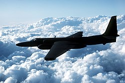
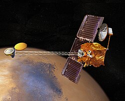
The TR-1 reconnaissance/surveillance aircraft

The 2001 Mars Odyssey used spectrometers and imagers to hunt for evidence of past or present water and volcanic activity on Mars.

The modern discipline of remote sensing arose with the development of flight. The balloonist G. Tournachon (alias Nadar) made photographs of Paris from his balloon in 1858. ^[50] Messenger pigeons, kites, rockets and unmanned balloons were also used for early images. With the exception of balloons, these first, individual images were not particularly useful for map making or for scientific purposes.

Systematic aerial photography was developed for military surveillance and reconnaissance purposes beginning in World War I. ^[51] After WWI, remote sensing technology was quickly adapted to civilian applications. ^[52] This is demonstrated by the first line of a 1941 textbook titled "Aerophotography and Aerosurverying," which stated the following:

"There is no longer any need to preach for aerial photography-not in the United States- for so widespread has become its use and so great its value that even the farmer who plants his fields in a remote corner of the country knows its value."

— James Bagley, ^[52]

The development of remote sensing technology reached a climax during the Cold War with the use of modified combat aircraft such as the P-51, P-38, RB-66 and the F-4C, or specifically designed collection platforms such as the U2/TR-1, SR-71, A-5 and the OV-1 series both in overhead and stand-off collection. ^[53] A more recent development is that of increasingly smaller sensor pods such as those used by law enforcement and the military, in both manned and unmanned platforms. The advantage of this approach is that this requires minimal modification to a given airframe. Later imaging technologies would include infrared, conventional, Doppler and synthetic aperture radar. ^[54]

The development of artificial satellites in the latter half of the 20th century allowed remote sensing to progress to a global scale as of the end of the Cold War. ^[55] Instrumentation aboard various Earth observing and weather satellites such as Landsat, the Nimbus and more recent missions such as RADARSAT and UARS provided global measurements of various data for civil, research, and military purposes. Space probes to other planets have also provided the opportunity to conduct remote sensing studies in extraterrestrial environments, synthetic aperture radar aboard the Magellan spacecraft provided detailed topographic maps of Venus, while instruments aboard SOHO allowed studies to be performed on the Sun and the solar wind, just to name a few examples. ^{[56] [57]}

Recent developments include, beginning in the 1960s and 1970s, the development of image processing of satellite imagery. The use of the term "remote sensing" began in the early 1960s when Evelyn Pruitt realized that advances in science meant that aerial photography was no longer an adequate term to describe the data streams being generated by new technologies. ^{[58] [59]} With assistance from her fellow staff member at the Office of Naval Research, Walter Bailey, she coined the term "remote sensing". ^{[60] [61]} Several research groups in Silicon Valley including NASA Ames Research Center, GTE, and ESL Inc. developed Fourier transform techniques leading to the first notable enhancement of imagery data. In 1999 the first commercial satellite (IKONOS) collecting very high resolution imagery was launched. ^[62]

Training and education

Remote Sensing has a growing relevance in the modern information society. It represents a key technology as part of the aerospace industry and bears increasing economic relevance – new sensors e.g. TerraSAR-X and RapidEye are developed constantly and the demand for skilled labour is increasing steadily. Furthermore, remote sensing exceedingly influences everyday life, ranging from weather forecasts to reports on climate change or natural disasters. As an example, 80% of the German students use the services of Google Earth; in 2006 alone the software was downloaded 100 million times. But studies have shown that only a fraction of them know more about the data they are working with. ^[63] There exists a huge knowledge gap between the application and the understanding of satellite images. Remote sensing only plays a tangential role in schools, regardless of the political claims to strengthen the support for teaching on the subject. ^[64] A lot of the computer software explicitly developed for school lessons has not yet been implemented due to its complexity. Thereby, the subject is either not at all integrated into the curriculum or does not pass the step of an interpretation of analogue images. In fact, the subject of remote sensing requires a consolidation of physics and mathematics as well as competences in the fields of media and methods apart from the mere visual interpretation of satellite images.

Many teachers have great interest in the subject "remote sensing", being motivated to integrate this topic into teaching, provided that the curriculum is considered. In many cases, this encouragement fails because of confusing information. ^[65] In order to integrate remote sensing in a sustainable manner organizations like the EGU or Digital Earth ^[66] encourage the development of learning modules and learning portals. Examples include: FIS – Remote Sensing in School Lessons, ^[67] Geospektiv, ^[68] Ychange, ^[69] or Spatial Discovery, ^[70] to promote media and method qualifications as well as independent learning.

Software

Main article: Remote sensing software

Remote sensing data are processed and analyzed with computer software, known as a remote sensing application. A large number of proprietary and open source applications exist to process remote sensing data.

Remote Sensing with gamma rays

There are applications of gamma rays to mineral exploration through remote sensing. In 1972 more than two million dollars were spent on remote sensing applications with gamma rays to mineral exploration. Gamma rays are used to search for deposits of uranium. By observing radioactivity from potassium, porphyry copper deposits can be located. A high ratio of uranium to thorium has been found to be related to the presence of hydrothermal copper deposits. Radiation patterns have also been known to occur above oil and gas fields, but some of these patterns were thought to be due to surface soils instead of oil and gas. ^[71]

Satellites

This section is an excerpt from Earth observation satellite.[ edit ]

Six Earth observation satellites comprising the A-train satellite constellation as of 2014.

An Earth observation satellite or Earth remote sensing satellite is a satellite used or designed for Earth observation (EO) from orbit, including spy satellites and similar ones intended for non-military uses such as environmental monitoring, meteorology, cartography and others. The most common type are Earth imaging satellites, that take satellite images, analogous to aerial photographs; some EO satellites may perform remote sensing without forming pictures, such as in GNSS radio occultation.

The first occurrence of satellite remote sensing can be dated to the launch of the first artificial satellite, Sputnik 1, by the Soviet Union on October 4, 1957. ^[72] Sputnik 1 sent back radio signals, which scientists used to study the ionosphere. ^[73] The United States Army Ballistic Missile Agency launched the first American satellite, Explorer 1, for NASA's Jet Propulsion Laboratory on January 31, 1958. The information sent back from its radiation detector led to the discovery of the Earth's Van Allen radiation belts. ^[74] The TIROS-1 spacecraft, launched on April 1, 1960, as part of NASA's Television Infrared Observation Satellite (TIROS) program, sent back the first television footage of weather patterns to be taken from space. ^[72]

In 2008, more than 150 Earth observation satellites were in orbit, recording data with both passive and active sensors and acquiring more than 10 terabits of data daily. ^[72] By 2021, that total had grown to over 950, with the largest number of satellites operated by US-based company Planet Labs. ^[75]

Most Earth observation satellites carry instruments that should be operated at a relatively low altitude. Most orbit at altitudes above 500 to 600 kilometers (310 to 370 mi). Lower orbits have significant air-drag, which makes frequent orbit reboost maneuvers necessary. The Earth observation satellites ERS-1, ERS-2 and Envisat of European Space Agency as well as the MetOp spacecraft of EUMETSAT are all operated at altitudes of about 800 km (500 mi). The Proba-1, Proba-2 and SMOS spacecraft of European Space Agency are observing the Earth from an altitude of about 700 km (430 mi). The Earth observation satellites of UAE, DubaiSat-1 & DubaiSat-2 are also placed in Low Earth Orbits (LEO) orbits and providing satellite imagery of various parts of the Earth. ^{[76] [77]}

To get global coverage with a low orbit, a polar orbit is used. A low orbit will have an orbital period of roughly 100 minutes and the Earth will rotate around its polar axis about 25° between successive orbits. The ground track moves towards the west 25° each orbit, allowing a different section of the globe to be scanned with each orbit. Most are in Sun-synchronous orbits.

A geostationary orbit, at 36,000 km (22,000 mi), allows a satellite to hover over a constant spot on the earth since the orbital period at this altitude is 24 hours. This allows uninterrupted coverage of more than 1/3 of the Earth per satellite, so three satellites, spaced 120° apart, can cover the whole Earth. This type of orbit is mainly used for meteorological satellites.

See also

Main category: Remote sensing

• Airborne Real-time Cueing Hyperspectral Enhanced Reconnaissance
• American Society for Photogrammetry and Remote Sensing
• Archaeological imagery
• Asian Association on Remote Sensing
• CLidar
• Coastal management
• Crateology
• First images of Earth from space
• Full spectral imaging
• Geographic information system (GIS)
• GIS and hydrology
• Geoinformatics
• Geophysical survey
• Global Positioning System (GPS)
• Ground truth § Remote sensing
• IEEE Geoscience and Remote Sensing Society
• Image mosaic
• Imagery analysis
• Imaging science
• International Society for Photogrammetry and Remote Sensing
• Land change science
• Liquid crystal tunable filter
• List of Earth observation satellites
• Mobile mapping
• Multispectral pattern recognition
• National Center for Remote Sensing, Air and Space Law
• National LIDAR Dataset
• Normalized difference water index
• Orthophoto
• Pictometry
• Radiometry
• Remote monitoring and control
• Technical geography
• TopoFlight
• Vector Map

References

1. Schowengerdt, Robert A. (2007). Remote sensing: models and methods for image processing (3rd ed.). Academic Press. p. 2. ISBN   978-0-12-369407-2. Archived from the original on 1 May 2016. Retrieved 15 November 2015.
2. Schott, John Robert (2007). Remote sensing: the image chain approach (2nd ed.). Oxford University Press. p. 1. ISBN   978-0-19-517817-3. Archived from the original on 24 April 2016. Retrieved 15 November 2015.
3. Guo, Huadong; Huang, Qingni; Li, Xinwu; Sun, Zhongchang; Zhang, Ying (2013). "Spatiotemporal analysis of urban environment based on the vegetation–impervious surface–soil model" (PDF). Journal of Applied Remote Sensing . 8: 084597. Bibcode:2014JARS....8.4597G. doi: 10.1117/1.JRS.8.084597 . S2CID   28430037. Archived (PDF) from the original on 19 July 2018. Retrieved 27 October 2021.
4. Liu, Jian Guo & Mason, Philippa J. (2009). Essential Image Processing for GIS and Remote Sensing. Wiley-Blackwell. p. 4. ISBN   978-0-470-51032-2 . Retrieved 2 April 2023.
5. "Saving the monkeys". SPIE Professional. Archived from the original on 4 February 2016. Retrieved 1 January 2016.
6. Howard, A.; et al. (19 August 2015). "Remote sensing and habitat mapping for bearded capuchin monkeys (Sapajus libidinosus): landscapes for the use of stone tools". Journal of Applied Remote Sensing. 9 (1): 096020. doi:10.1117/1.JRS.9.096020. S2CID   120031016.
7. Innocenti, Fabrizio; Robinson, Rod; Gardiner, Tom; Finlayson, Andrew; Connor, Andy (2017). "Differential Absorption Lidar (DIAL) Measurements of Landfill Methane Emissions". Remote Sensing. 9 (9): 953. Bibcode:2017RemS....9..953I. doi: 10.3390/rs9090953 .
8. C. Bayindir; J. D. Frost; C. F. Barnes (January 2018). "Assessment and enhancement of SAR noncoherent change detection of sea-surface oil spills". IEEE J. Ocean. Eng. 43 (1): 211–220. Bibcode:2018IJOE...43..211B. doi:10.1109/JOE.2017.2714818. S2CID   44706251.
9. "Science@nasa - Technology: Remote Sensing". Archived from the original on 29 September 2006. Retrieved 18 February 2009.
10. Zhao, Kaiguang; Suarez, Juan C; Garcia, Mariano; Hu, Tongxi; Wang, Cheng; Londo, Alexis (2018). "Utility of multitemporal lidar for forest and carbon monitoring: Tree growth, biomass dynamics, and carbon flux". Remote Sensing of Environment. 204: 883–897. Bibcode:2018RSEnv.204..883Z. doi:10.1016/j.rse.2017.09.007.
11. Just Sit Right Back and You'll Hear a Tale, a Tale of a Plankton Trip Archived 10 August 2021 at the Wayback Machine NASA Earth Expeditions, 15 August 2018.
12. Levin, Noam; Kyba, Christopher C.M.; Zhang, Qingling; Sánchez de Miguel, Alejandro; Román, Miguel O.; Li, Xi; Portnov, Boris A.; Molthan, Andrew L.; Jechow, Andreas; Miller, Steven D.; Wang, Zhuosen; Shrestha, Ranjay M.; Elvidge, Christopher D. (February 2020). "Remote sensing of night lights: A review and an outlook for the future". Remote Sensing of Environment. 237: 111443. Bibcode:2020RSEnv.23711443L. doi:10.1016/j.rse.2019.111443. hdl: 10871/40052 . S2CID   214254543.
13. Corradino, Claudia; Ganci, Gaetana; Bilotta, Giuseppe; Cappello, Annalisa; Del Negro, Ciro; Fortuna, Luigi (January 2019). "Smart Decision Support Systems for Volcanic Applications". Energies. 12 (7): 1216. doi: 10.3390/en12071216 .
14. Corradino, Claudia; Ganci, Gaetana; Cappello, Annalisa; Bilotta, Giuseppe; Hérault, Alexis; Del Negro, Ciro (January 2019). "Mapping Recent Lava Flows at Mount Etna Using Multispectral Sentinel-2 Images and Machine Learning Techniques". Remote Sensing. 11 (16): 1916. Bibcode:2019RemS...11.1916C. doi: 10.3390/rs11161916 .
15. Goldberg, A.; Stann, B.; Gupta, N. (July 2003). "Multispectral, Hyperspectral, and Three-Dimensional Imaging Research at the U.S. Army Research Laboratory" (PDF). Proceedings of the International Conference on International Fusion [6th]. 1: 499–506.
16. Makki, Ihab; Younes, Rafic; Francis, Clovis; Bianchi, Tiziano; Zucchetti, Massimo (1 February 2017). "A survey of landmine detection using hyperspectral imaging". ISPRS Journal of Photogrammetry and Remote Sensing. 124: 40–53. Bibcode:2017JPRS..124...40M. doi:10.1016/j.isprsjprs.2016.12.009. ISSN   0924-2716.
17. Mills, J.P.; et al. (1997). "Photogrammetry from Archived Digital Imagery for Seal Monitoring". The Photogrammetric Record. 15 (89): 715–724. doi:10.1111/0031-868X.00080. S2CID   140189982.
18. Twiss, S.D.; et al. (2001). "Topographic spatial characterisation of grey seal Halichoerus grypus breeding habitat at a sub-seal size spatial grain". Ecography. 24 (3): 257–266. doi: 10.1111/j.1600-0587.2001.tb00198.x .
19. Stewart, J.E.; et al. (2014). "Finescale ecological niche modeling provides evidence that lactating gray seals (Halichoerus grypus) prefer access to fresh water in order to drink" (PDF). Marine Mammal Science. 30 (4): 1456–1472. Bibcode:2014MMamS..30.1456S. doi:10.1111/mms.12126. Archived (PDF) from the original on 13 July 2021. Retrieved 27 October 2021.
20. Zhang, Chuanrong; Li, Xinba (September 2022). "Land Use and Land Cover Mapping in the Era of Big Data". Land. 11 (10): 1692. doi: 10.3390/land11101692 .
21. "Begni G. Escadafal R. Fontannaz D. and Hong-Nga Nguyen A.-T. (2005). Remote sensing: a tool to monitor and assess desertification. Les dossiers thématiques du CSFD. Issue 2. 44 pp". Archived from the original on 26 May 2019. Retrieved 27 October 2021.
22. Wang, Ran; Gamon, John A. (15 September 2019). "Remote sensing of terrestrial plant biodiversity". Remote Sensing of Environment. 231: 111218. Bibcode:2019RSEnv.23111218W. doi:10.1016/j.rse.2019.111218. ISSN   0034-4257. S2CID   197567301.
23. Rocchini, Duccio; Boyd, Doreen S.; Féret, Jean-Baptiste; Foody, Giles M.; He, Kate S.; Lausch, Angela; Nagendra, Harini; Wegmann, Martin; Pettorelli, Nathalie (February 2016). Skidmore, Andrew; Chauvenet, Alienor (eds.). "Satellite remote sensing to monitor species diversity: potential and pitfalls". Remote Sensing in Ecology and Conservation. 2 (1): 25–36. Bibcode:2016RSEC....2...25R. doi:10.1002/rse2.9. hdl: 11585/720672 . ISSN   2056-3485. S2CID   59446258.
24. Schweiger, Anna K.; Cavender-Bares, Jeannine; Townsend, Philip A.; Hobbie, Sarah E.; Madritch, Michael D.; Wang, Ran; Tilman, David; Gamon, John A. (June 2018). "Plant spectral diversity integrates functional and phylogenetic components of biodiversity and predicts ecosystem function". Nature Ecology & Evolution. 2 (6): 976–982. Bibcode:2018NatEE...2..976S. doi:10.1038/s41559-018-0551-1. ISSN   2397-334X. PMID   29760440. S2CID   256718584.
25. Cerrejón, Carlos; Valeria, Osvaldo; Marchand, Philippe; Caners, Richard T.; Fenton, Nicole J. (18 February 2021). "No place to hide: Rare plant detection through remote sensing". Diversity and Distributions. 27 (6): 948–961. Bibcode:2021DivDi..27..948C. doi: 10.1111/ddi.13244 . ISSN   1366-9516. S2CID   233886263.
26. Carfagna, E. (2005). "Using remote sensing for agricultural statistics". International Statistical Review. 73 (3): 389–404. doi:10.1111/j.1751-5823.2005.tb00155.x.
27. "Geodetic Imaging". Archived from the original on 2 October 2016. Retrieved 29 September 2016.
28. Grigoriev А.N. (2015). "Мethod of radiometric distortion correction of multispectral data for the earth remote sensing". Scientific and Technical Journal of Information Technologies, Mechanics and Optics. 15 (4): 595–602. doi: 10.17586/2226-1494-2015-15-4-595-602 .
29. NASA (1986), Report of the EOS data panel, Earth Observing System, Data and Information System, Data Panel Report, Vol. IIa., NASA Technical Memorandum 87777, June 1986, 62 pp. Available at http://hdl.handle.net/2060/19860021622 Archived 27 October 2021 at the Wayback Machine
30. C. L. Parkinson, A. Ward, M. D. King (Eds.) Earth Science Reference Handbook – A Guide to NASA's Earth Science Program and Earth Observing Satellite Missions, National Aeronautics and Space Administration Washington, D. C. Available at http://eospso.gsfc.nasa.gov/ftp_docs/2006ReferenceHandbook.pdf Archived 15 April 2010 at the Wayback Machine
31. GRAS-SAF (2009), Product User Manual, GRAS Satellite Application Facility, Version 1.2.1, 31 March 2009. Available at http://www.grassaf.org/general-documents/products/grassaf_pum_v121.pdf Archived 26 July 2011 at the Wayback Machine
32. Houston, A.H. "Use of satellite data in agricultural surveys". Communications in Statistics. Theory and Methods (23): 2857–2880.
33. Allen, J.D. "A Look at the Remote Sensing Applications Program of the National Agricultural Statistics Service". Journal of Official Statistics. 6 (4): 393–409.
34. Taylor, J (1997). Regional Crop Inventories in Europe Assisted by Remote Sensing: 1988-1993. Synthesis Report. Luxembourg: Office for Pubblications of the EC.
35. Foody, G.M. (1994). "Estimation of tropical forest extent and regenerative stage using remotely sensed data". Journal of Biogeography. 21 (3): 223–244. Bibcode:1994JBiog..21..223F. doi:10.2307/2845527. JSTOR   2845527.
36. Achard, F (2002). "Determination of deforestation rates of the world's humid tropical forests". Science. 297 (5583): 999–1002. Bibcode:2002Sci...297..999A. doi:10.1126/science.1070656. PMID   12169731.
37. Ambrosio Flores, L (2000). "Land cover estimation in small areas using ground survey and remote sensing". Remote Sensing of the Environment. 74 (2): 240–248. Bibcode:2000RSEnv..74..240F. doi:10.1016/S0034-4257(00)00114-0.
38. Green, Russell G. Congalton, Kass (25 January 2019). Assessing the Accuracy of Remotely Sensed Data: Principles and Practices, Third Edition (3 ed.). Boca Raton: CRC Press. doi:10.1201/9780429052729. ISBN   978-0-429-05272-9.
39. Stehman, S. (2013). "Estimating Area from an Accuracy Assessment Error Matrix". Remote Sensing of Environment. 132 (132): 202–211. Bibcode:2013RSEnv.132..202S. doi:10.1016/j.rse.2013.01.016.
40. Stehman, S. (2019). "Key issues in rigorous accuracy assessment of land cover products". Remote Sensing of Environment. 231 (231). Bibcode:2019RSEnv.23111199S. doi:10.1016/j.rse.2019.05.018.
41. Zhen, Z (2013). "Impact of training and validation sample selection on classification accuracy and accuracy assessment when using reference polygons in object-based classification". International Journal of Remote Sensing. 34 (19): 6914–6930. Bibcode:2013IJRS...34.6914Z. doi:10.1080/01431161.2013.810822.
42. Czaplewski, R.L. "Misclassification bias in areal estimates". Photogrammetric Engineering and Remote Sensing (39): 189–192.
43. Bauer, M.E. (1978). "Area estimation of crops by digital analysis of Landsat data". Photogrammetric Engineering and Remote Sensing (44): 1033–1043.
44. Olofsson, P. (2014). "Good practices for estimating area and assessing accuracy of land change". Remote Sensing of Environment. 148 (148): 42–57. Bibcode:2014RSEnv.148...42O. doi:10.1016/j.rse.2014.02.015.
45. Mcroberts, R (2018). "The effects of imperfect reference data on remote sensing-assisted estimators of land cover class proportions". ISPRS Journal of Photogrammetry and Remote Sensing. 142 (142): 292–300. Bibcode:2018JPRS..142..292M. doi: 10.1016/j.isprsjprs.2018.06.002 .
46. Foody, G.M. (2010). "Assessing the accuracy of land cover change with imperfect ground reference data". Remote Sensing of Environment. 114 (10): 2271–2285. Bibcode:2010RSEnv.114.2271F. doi:10.1016/j.rse.2010.05.003.
47. Sannier, C (2014). "Using the regression estimator with landsat data to estimate proportion forest cover and net proportion deforestation in gabon". Remote Sensing of Environment. 151 (151): 138–148. Bibcode:2014RSEnv.151..138S. doi:10.1016/j.rse.2013.09.015.
48. Gallego, F.J. (2004). "Remote sensing and land cover area estimation". International Journal of Remote Sensing. 25 (5): 3019–3047. Bibcode:2004IJRS...25.3019G. doi:10.1080/01431160310001619607.
49. Carfagna, E. (2005). "Using remote sensing for agricultural statistics". International Statistical Review. 73 (3): 389–404. doi:10.1111/j.1751-5823.2005.tb00155.x.
50. Maksel, Rebecca. "Flight of the Giant". Air & Space Magazine. Archived from the original on 18 August 2021. Retrieved 19 February 2019.
51. IWM, Alan Wakefield
    Head of photographs at (4 April 2014). "A bird's-eye view of the battlefield: aerial photography". The Daily Telegraph. ISSN   0307-1235. Archived from the original on 18 April 2014. Retrieved 19 February 2019.
52. Bagley, James (1941). Aerophotography and Aerosurverying (1st ed.). York, PA: The Maple Press Company.
53. "Air Force Magazine". www.airforcemag.com. Archived from the original on 19 February 2019. Retrieved 19 February 2019.
54. "Military Imaging and Surveillance Technology (MIST)". www.darpa.mil. Archived from the original on 18 August 2021. Retrieved 19 February 2019.
55. The Indian Society of International Law - Newsletter: VOL. 15, No. 4, October - December 2016 (Report). doi:10.1163/2210-7975_hrd-9920-2016004.
56. "In Depth | Magellan". Solar System Exploration: NASA Science. Archived from the original on 19 October 2021. Retrieved 19 February 2019.
57. Garner, Rob (15 April 2015). "SOHO - Solar and Heliospheric Observatory". NASA. Archived from the original on 18 September 2021. Retrieved 19 February 2019.
58. Campbell, James B.; Wynne, Randolph H. (21 June 2011). Introduction to Remote Sensing (5th ed.). New York London: The Guilford Press. ISBN   978-1-60918-176-5.
59. Ryerson, Robert A. (2010). Why 'where' matters : understanding and profiting from GPS, GIS, and remote sensing : practical advice for individuals, communities, companies and countries. Internet Archive. Manotick, ON : Kim Geomatics Corp. ISBN   978-0-9866376-0-5.
60. Fussell, Jay; Rundquist, Donald; Harrington, John A. (September 1986). "On defining remote sensing" (PDF). Photogrammetric Engineering and Remote Sensing. 52 (9): 1507–1511. Archived from the original (PDF) on 4 October 2021.
61. Pruitt, Evelyn L. (1979). "The Office of Naval Research and Geography". Annals of the Association of American Geographers. 69 (1): 103–108. doi:10.1111/j.1467-8306.1979.tb01235.x. ISSN   0004-5608. JSTOR   2569553.
62. Colen, Jerry (8 April 2015). "Ames Research Center Overview". NASA. Archived from the original on 28 September 2021. Retrieved 19 February 2019.
63. Ditter, R., Haspel, M., Jahn, M., Kollar, I., Siegmund, A., Viehrig, K., Volz, D., Siegmund, A. (2012) Geospatial technologies in school – theoretical concept and practical implementation in K-12 schools. In: International Journal of Data Mining, Modelling and Management (IJDMMM): FutureGIS: Riding the Wave of a Growing Geospatial Technology Literate Society; Vol. X
64. Stork, E.J., Sakamoto, S.O., and Cowan, R.M. (1999) "The integration of science explorations through the use of earth images in middle school curriculum", Proc. IEEE Trans. Geosci. Remote Sensing 37, 1801–1817
65. Bednarz, S.W.; Whisenant, S.E. (July 2000). "Mission Geography: Linking national geography standards, innovative technologies and NASA". IGARSS 2000. IEEE 2000 International Geoscience and Remote Sensing Symposium. Taking the Pulse of the Planet: The Role of Remote Sensing in Managing the Environment. Proceedings (Cat. No.00CH37120). Vol. 6. pp. 2780–2782 vol.6. doi:10.1109/IGARSS.2000.859713. ISBN   0-7803-6359-0. S2CID   62414447.
66. Digital Earth
67. "FIS – Remote Sensing in School Lessons". Archived from the original on 26 October 2012. Retrieved 25 October 2012.
68. "geospektiv". Archived from the original on 2 May 2018. Retrieved 1 June 2018.
69. "YCHANGE". Archived from the original on 17 August 2018. Retrieved 1 June 2018.
70. "Landmap – Spatial Discovery". Archived from the original on 29 November 2014. Retrieved 27 October 2021.
71. Grasty, R (1976). Applications of Gamma Radiation in Remote Sensing (1st ed.). Berlin: Springer-Verlag. p. 267. ISBN   978-3-642-66238-6.
72. Tatem, Andrew J.; Goetz, Scott J.; Hay, Simon I. (2008). "Fifty Years of Earth-observation Satellites". American Scientist. 96 (5): 390–398. doi:10.1511/2008.74.390. PMC   2690060 . PMID   19498953.
73. Kuznetsov, V.D.; Sinelnikov, V.M.; Alpert, S.N. (June 2015). "Yakov Alpert: Sputnik-1 and the first satellite ionospheric experiment". Advances in Space Research. 55 (12): 2833–2839. Bibcode:2015AdSpR..55.2833K. doi:10.1016/j.asr.2015.02.033.
74. "James A. Van Allen". nmspacemuseum.org. New Mexico Museum of Space History. Retrieved 14 May 2018.
75. "How many Earth observation satellites are orbiting the planet in 2021?". 18 August 2021.
76. "DubaiSat-2, Earth Observation Satellite of UAE". Mohammed Bin Rashid Space Centre. Archived from the original on 17 January 2019. Retrieved 4 July 2016.
77. "DubaiSat-1, Earth Observation Satellite of UAE". Mohammed Bin Rashid Space Centre. Archived from the original on 4 March 2016. Retrieved 4 July 2016.

Further reading

• Campbell, J. B. (2002). Introduction to remote sensing (3rd ed.). The Guilford Press. ISBN   978-1-57230-640-0.
• Datla, R.U.; Rice, J.P.; Lykke, K.R.; Johnson, B.C.; Butler, J.J.; Xiong, X. (March–April 2011). "Best practice guidelines for pre-launch characterization and calibration of instruments for passive optical remote sensing". Journal of Research of the National Institute of Standards and Technology. 116 (2): 612–646. doi:10.6028/jres.116.009. PMC   4550341 . PMID   26989588.
• Dupuis, C.; Lejeune, P.; Michez, A.; Fayolle, A. How Can Remote Sensing Help Monitor Tropical Moist Forest Degradation?—A Systematic Review. Remote Sens. 2020, 12, 1087. https://www.mdpi.com/2072-4292/12/7/1087
• Jensen, J. R. (2007). Remote sensing of the environment: an Earth resource perspective (2nd ed.). Prentice Hall. ISBN   978-0-13-188950-7.
• Jensen, J. R. (2005). Digital Image Processing: a Remote Sensing Perspective (3rd ed.). Prentice Hall.
• KUENZER, C. ZHANG, J., TETZLAFF, A., and S. DECH, 2013: Thermal Infrared Remote Sensing of Surface and underground Coal Fires. In (eds.) Kuenzer, C. and S. Dech 2013: Thermal Infrared Remote Sensing – Sensors, Methods, Applications. Remote Sensing and Digital Image Processing Series, Volume 17, 572 pp., ISBN   978-94-007-6638-9, pp. 429–451
• Kuenzer, C. and S. Dech 2013: Thermal Infrared Remote Sensing – Sensors, Methods, Applications. Remote Sensing and Digital Image Processing Series, Volume 17, 572 pp., ISBN   978-94-007-6638-9
• Lasaponara, R. and Masini N. 2012: Satellite Remote Sensing - A new tool for Archaeology. Remote Sensing and Digital Image Processing Series, Volume 16, 364 pp., ISBN   978-90-481-8801-7.
• Lentile, Leigh B.; Holden, Zachary A.; Smith, Alistair M. S.; Falkowski, Michael J.; Hudak, Andrew T.; Morgan, Penelope; Lewis, Sarah A.; Gessler, Paul E.; Benson, Nate C. (2006). "Remote sensing techniques to assess active fire characteristics and post-fire effects". International Journal of Wildland Fire. 3 (15): 319–345. doi:10.1071/WF05097. S2CID   724358. Archived from the original on 12 August 2014. Retrieved 4 February 2010.
• Lillesand, T. M.; R. W. Kiefer; J. W. Chipman (2003). Remote sensing and image interpretation (5th ed.). Wiley. ISBN   978-0-471-15227-9.
• Richards, J. A.; X. Jia (2006). Remote sensing digital image analysis: an introduction (4th ed.). Springer. ISBN   978-3-540-25128-6.

External links

• Media related to Remote sensing at Wikimedia Commons
• Remote Sensing at Curlie