Last updated Mathematical models developed in theoretical ecology predict complex food webs can be less stable than simpler webs.Life on Earth-Flow of Energy and Entropy
Theoretical ecology is the scientific discipline devoted to the study of ecological systems using theoretical methods such as simple conceptual models, mathematical models, computational simulations, and advanced data analysis. Effective models improve understanding of the natural world by revealing how the dynamics of species populations are often based on fundamental biological conditions and processes. Further, the field aims to unify a diverse range of empirical observations by assuming that common, mechanistic processes generate observable phenomena across species and ecological environments. Based on biologically realistic assumptions, theoretical ecologists are able to uncover novel, non-intuitive insights about natural processes. Theoretical results are often verified by empirical and observational studies, revealing the power of theoretical methods in both predicting and understanding the noisy, diverse biological world.
The field is broad and includes foundations in applied mathematics, computer science, biology, statistical physics, genetics, chemistry, evolution, and conservation biology. Theoretical ecology aims to explain a diverse range of phenomena in the life sciences, such as population growth and dynamics, fisheries, competition, evolutionary theory, epidemiology, animal behavior and group dynamics, food webs, ecosystems, spatial ecology, and the effects of climate change.
Theoretical ecology has further benefited from the advent of fast computing power, allowing the analysis and visualization of large-scale computational simulations of ecological phenomena. Importantly, these modern tools provide quantitative predictions about the effects of human induced environmental change on a diverse variety of ecological phenomena, such as: species invasions, climate change, the effect of fishing and hunting on food network stability, and the global carbon cycle.
Modelling approaches
As in most other sciences, mathematical models form the foundation of modern ecological theory.
Phenomenological models: distill the functional and distributional shapes from observed patterns in the data, or researchers decide on functions and distribution that are flexible enough to match the patterns they or others (field or experimental ecologists) have found in the field or through experimentation.[3]
Mechanistic models: model the underlying processes directly, with functions and distributions that are based on theoretical reasoning about ecological processes of interest.[3]
Deterministic models always evolve in the same way from a given starting point.[4] They represent the average, expected behavior of a system, but lack random variation. Many system dynamics models are deterministic.
Stochastic models allow for the direct modeling of the random perturbations that underlie real world ecological systems. Markov chain models are stochastic.
Discrete time is modelled using difference equations. These model ecological processes that can be described as occurring over discrete time steps. Matrix algebra is often used to investigate the evolution of age-structured or stage-structured populations. The Leslie matrix, for example, mathematically represents the discrete time change of an age structured population.[6][7][8]
Models are often used to describe real ecological reproduction processes of single or multiple species. These can be modelled using stochastic branching processes. Examples are the dynamics of interacting populations (predationcompetition and mutualism), which, depending on the species of interest, may best be modeled over either continuous or discrete time. Other examples of such models may be found in the field of mathematical epidemiology where the dynamic relationships that are to be modeled are host–pathogen interactions.[5]
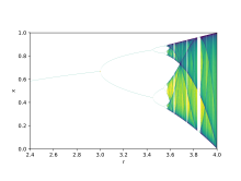
Bifurcation diagram of the logistic map
Bifurcation theory is used to illustrate how small changes in parameter values can give rise to dramatically different long run outcomes, a mathematical fact that may be used to explain drastic ecological differences that come about in qualitatively very similar systems.[9]Logistic maps are polynomial mappings, and are often cited as providing archetypal examples of how chaotic behaviour can arise from very simple non-linear dynamical equations. The maps were popularized in a seminal 1976 paper by the theoretical ecologist Robert May.[10] The difference equation is intended to capture the two effects of reproduction and starvation.
In 1930, R.A. Fisher published his classic The Genetical Theory of Natural Selection, which introduced the idea that frequency-dependent fitness brings a strategic aspect to evolution, where the payoffs to a particular organism, arising from the interplay of all of the relevant organisms, are the number of this organism' s viable offspring.[11] In 1961, Richard Lewontin applied game theory to evolutionary biology in his Evolution and the Theory of Games,[12] followed closely by John Maynard Smith, who in his seminal 1972 paper, “Game Theory and the Evolution of Fighting",[13] defined the concept of the evolutionarily stable strategy.
Because ecological systems are typically nonlinear, they often cannot be solved analytically and in order to obtain sensible results, nonlinear, stochastic and computational techniques must be used. One class of computational models that is becoming increasingly popular are the agent-based models. These models can simulate the actions and interactions of multiple, heterogeneous, organisms where more traditional, analytical techniques are inadequate. Applied theoretical ecology yields results which are used in the real world. For example, optimal harvesting theory draws on optimization techniques developed in economics, computer science and operations research, and is widely used in fisheries.[14]
Population ecology is a sub-field of ecology that deals with the dynamics of speciespopulations and how these populations interact with the environment.[15] It is the study of how the population sizes of species living together in groups change over time and space, and was one of the first aspects of ecology to be studied and modelled mathematically.
The most basic way of modeling population dynamics is to assume that the rate of growth of a population depends only upon the population size at that time and the per capita growth rate of the organism. In other words, if the number of individuals in a population at a time t, is N(t), then the rate of population growth is given by:
where r is the per capita growth rate, or the intrinsic growth rate of the organism. It can also be described as r = b-d, where b and d are the per capita time-invariant birth and death rates, respectively. This first orderlinear differential equation can be solved to yield the solution
,
a trajectory known as Malthusian growth, after Thomas Malthus, who first described its dynamics in 1798. A population experiencing Malthusian growth follows an exponential curve, where N(0) is the initial population size. The population grows when r > 0, and declines when r < 0. The model is most applicable in cases where a few organisms have begun a colony and are rapidly growing without any limitations or restrictions impeding their growth (e.g. bacteria inoculated in rich media).
The exponential growth model makes a number of assumptions, many of which often do not hold. For example, many factors affect the intrinsic growth rate and is often not time-invariant. A simple modification of the exponential growth is to assume that the intrinsic growth rate varies with population size. This is reasonable: the larger the population size, the fewer resources available, which can result in a lower birth rate and higher death rate. Hence, we can replace the time-invariant r with r’(t) = (b –a*N(t)) – (d + c*N(t)), where a and c are constants that modulate birth and death rates in a population dependent manner (e.g. intraspecific competition). Both a and c will depend on other environmental factors which, we can for now, assume to be constant in this approximated model. The differential equation is now:[16]
The biological significance of K becomes apparent when stabilities of the equilibria of the system are considered. The constant K is the carrying capacity of the population. The equilibria of the system are N = 0 and N = K. If the system is linearized, it can be seen that N = 0 is an unstable equilibrium while K is a stable equilibrium.[16]
Another assumption of the exponential growth model is that all individuals within a population are identical and have the same probabilities of surviving and of reproducing. This is not a valid assumption for species with complex life histories. The exponential growth model can be modified to account for this, by tracking the number of individuals in different age classes (e.g. one-, two-, and three-year-olds) or different stage classes (juveniles, sub-adults, and adults) separately, and allowing individuals in each group to have their own survival and reproduction rates. The general form of this model is
where Nt is a vector of the number of individuals in each class at time t and L is a matrix that contains the survival probability and fecundity for each class. The matrix L is referred to as the Leslie matrix for age-structured models, and as the Lefkovitch matrix for stage-structured models.[17]
If parameter values in L are estimated from demographic data on a specific population, a structured model can then be used to predict whether this population is expected to grow or decline in the long-term, and what the expected age distribution within the population will be. This has been done for a number of species including loggerhead sea turtles and right whales.[18][19]
An ecological community is a group of trophically similar, sympatric species that actually or potentially compete in a local area for the same or similar resources.[20] Interactions between these species form the first steps in analyzing more complex dynamics of ecosystems. These interactions shape the distribution and dynamics of species. Of these interactions, predation is one of the most widespread population activities.[21] Taken in its most general sense, predation comprises predator–prey, host–pathogen, and host–parasitoid interactions.
Lotka–Volterra model of cheetah–baboon interactions. Starting with 80 baboons (green) and 40 cheetahs, this graph shows how the model predicts the two species numbers will progress over time.
Predator–prey interaction
Predator–prey interactions exhibit natural oscillations in the populations of both predator and the prey.[21] In 1925, the American mathematician Alfred J. Lotka developed simple equations for predator–prey interactions in his book on biomathematics.[22] The following year, the Italian mathematician Vito Volterra, made a statistical analysis of fish catches in the Adriatic[23] and independently developed the same equations.[24] It is one of the earliest and most recognised ecological models, known as the Lotka-Volterra model:
where N is the prey and P is the predator population sizes, r is the rate for prey growth, taken to be exponential in the absence of any predators, α is the prey mortality rate for per-capita predation (also called ‘attack rate’), c is the efficiency of conversion from prey to predator, and d is the exponential death rate for predators in the absence of any prey.
Volterra originally used the model to explain fluctuations in fish and shark populations after fishing was curtailed during the First World War. However, the equations have subsequently been applied more generally.[25] Other examples of these models include the Lotka-Volterra model of the snowshoe hare and Canadian lynx in North America,[26] any infectious disease modeling such as the recent outbreak of SARS[27] and biological control of California red scale by the introduction of its parasitoid, Aphytis melinus .[28]
A credible, simple alternative to the Lotka-Volterra predator–prey model and their common prey dependent generalizations is the ratio dependent or Arditi-Ginzburg model.[29] The two are the extremes of the spectrum of predator interference models. According to the authors of the alternative view, the data show that true interactions in nature are so far from the Lotka–Volterra extreme on the interference spectrum that the model can simply be discounted as wrong. They are much closer to the ratio-dependent extreme, so if a simple model is needed one can use the Arditi–Ginzburg model as the first approximation.[30]
The second interaction, that of host and pathogen, differs from predator–prey interactions in that pathogens are much smaller, have much faster generation times, and require a host to reproduce. Therefore, only the host population is tracked in host–pathogen models. Compartmental models that categorize host population into groups such as susceptible, infected, and recovered (SIR) are commonly used.[31]
Host–parasitoid interaction
The third interaction, that of host and parasitoid, can be analyzed by the Nicholson–Bailey model, which differs from Lotka-Volterra and SIR models in that it is discrete in time. This model, like that of Lotka-Volterra, tracks both populations explicitly. Typically, in its general form, it states:
where f(Nt, Pt) describes the probability of infection (typically, Poisson distribution), λ is the per-capita growth rate of hosts in the absence of parasitoids, and c is the conversion efficiency, as in the Lotka-Volterra model.[21]
Competition and mutualism
In studies of the populations of two species, the Lotka-Volterra system of equations has been extensively used to describe dynamics of behavior between two species, N1 and N2. Examples include relations between D. discoiderum and E. coli,[32] as well as theoretical analysis of the behavior of the system.[33]
The r coefficients give a “base” growth rate to each species, while K coefficients correspond to the carrying capacity. What can really change the dynamics of a system, however are the α terms. These describe the nature of the relationship between the two species. When α12 is negative, it means that N2 has a negative effect on N1, by competing with it, preying on it, or any number of other possibilities. When α12 is positive, however, it means that N2 has a positive effect on N1, through some kind of mutualistic interaction between the two. When both α12 and α21 are negative, the relationship is described as competitive. In this case, each species detracts from the other, potentially over competition for scarce resources. When both α12 and α21 are positive, the relationship becomes one of mutualism. In this case, each species provides a benefit to the other, such that the presence of one aids the population growth of the other.
Unified neutral theory is a hypothesis proposed by Stephen P. Hubbell in 2001.[20] The hypothesis aims to explain the diversity and relative abundance of species in ecological communities, although like other neutral theories in ecology, Hubbell's hypothesis assumes that the differences between members of an ecological community of trophically similar species are "neutral," or irrelevant to their success. Neutrality means that at a given trophic level in a food web, species are equivalent in birth rates, death rates, dispersal rates and speciation rates, when measured on a per-capita basis.[34] This implies that biodiversity arises at random, as each species follows a random walk.[35] This can be considered a null hypothesis to niche theory. The hypothesis has sparked controversy, and some authors consider it a more complex version of other null models that fit the data better.
Under unified neutral theory, complex ecological interactions are permitted among individuals of an ecological community (such as competition and cooperation), providing all individuals obey the same rules. Asymmetric phenomena such as parasitism and predation are ruled out by the terms of reference; but cooperative strategies such as swarming, and negative interaction such as competing for limited food or light are allowed, so long as all individuals behave the same way. The theory makes predictions that have implications for the management of biodiversity, especially the management of rare species. It predicts the existence of a fundamental biodiversity constant, conventionally written θ, that appears to govern species richness on a wide variety of spatial and temporal scales.
Biogeography is the study of the distribution of species in space and time. It aims to reveal where organisms live, at what abundance, and why they are (or are not) found in a certain geographical area.
Biogeography is most keenly observed on islands, which has led to the development of the subdiscipline of island biogeography. These habitats are often a more manageable areas of study because they are more condensed than larger ecosystems on the mainland. In 1967, Robert MacArthur and E.O. Wilson published The Theory of Island Biogeography. This showed that the species richness in an area could be predicted in terms of factors such as habitat area, immigration rate and extinction rate.[36] The theory is considered one of the fundamentals of ecological theory.[37] The application of island biogeography theory to habitat fragments spurred the development of the fields of conservation biology and landscape ecology.[38]
A population ecology concept is r/K selection theory, one of the first predictive models in ecology used to explain life-history evolution. The premise behind the r/K selection model is that natural selection pressures change according to population density. For example, when an island is first colonized, density of individuals is low. The initial increase in population size is not limited by competition, leaving an abundance of available resources for rapid population growth. These early phases of population growth experience density-independent forces of natural selection, which is called r-selection. As the population becomes more crowded, it approaches the island's carrying capacity, thus forcing individuals to compete more heavily for fewer available resources. Under crowded conditions, the population experiences density-dependent forces of natural selection, called K-selection.[39][40]
Spatial analysis of ecological systems often reveals that assumptions that are valid for spatially homogenous populations – and indeed, intuitive – may no longer be valid when migratory subpopulations moving from one patch to another are considered.[42] In a simple one-species formulation, a subpopulation may occupy a patch, move from one patch to another empty patch, or die out leaving an empty patch behind. In such a case, the proportion of occupied patches may be represented as
where m is the rate of colonization, and e is the rate of extinction.[43] In this model, if e < m, the steady state value of p is 1 – (e/m) while in the other case, all the patches will eventually be left empty. This model may be made more complex by addition of another species in several different ways, including but not limited to game theoretic approaches, predator–prey interactions, etc. We will consider here an extension of the previous one-species system for simplicity. Let us denote the proportion of patches occupied by the first population as p1, and that by the second as p2. Then,
In this case, if e is too high, p1 and p2 will be zero at steady state. However, when the rate of extinction is moderate, p1 and p2 can stably coexist. The steady state value of p2 is given by
(p*1 may be inferred by symmetry). If e is zero, the dynamics of the system favor the species that is better at colonizing (i.e. has the higher m value). This leads to a very important result in theoretical ecology known as the Intermediate Disturbance Hypothesis, where the biodiversity (the number of species that coexist in the population) is maximized when the disturbance (of which e is a proxy here) is not too high or too low, but at intermediate levels.[44]
The form of the differential equations used in this simplistic modelling approach can be modified. For example:
Colonization may be dependent on p linearly (m*(1-p)) as opposed to the non-linear m*p*(1-p) regime described above. This mode of replication of a species is called the “rain of propagules”, where there is an abundance of new individuals entering the population at every generation. In such a scenario, the steady state where the population is zero is usually unstable.[45]
Extinction may depend non-linearly on p (e*p*(1-p)) as opposed to the linear (e*p) regime described above. This is referred to as the “rescue effect” and it is again harder to drive a population extinct under this regime.[45]
The model can also be extended to combinations of the four possible linear or non-linear dependencies of colonization and extinction on p are described in more detail in.[46]
Introducing new elements, whether biotic or abiotic, into ecosystems can be disruptive. In some cases, it leads to ecological collapse, trophic cascades and the death of many species within the ecosystem. The abstract notion of ecological health attempts to measure the robustness and recovery capacity for an ecosystem; i.e. how far the ecosystem is away from its steady state. Often, however, ecosystems rebound from a disruptive agent. The difference between collapse or rebound depends on the toxicity of the introduced element and the resiliency of the original ecosystem.
If ecosystems are governed primarily by stochastic processes, through which its subsequent state would be determined by both predictable and random actions, they may be more resilient to sudden change than each species individually. In the absence of a balance of nature, the species composition of ecosystems would undergo shifts that would depend on the nature of the change, but entire ecological collapse would probably be infrequent events. In 1997, Robert Ulanowicz used information theory tools to describe the structure of ecosystems, emphasizing mutual information (correlations) in studied systems. Drawing on this methodology and prior observations of complex ecosystems, Ulanowicz depicts approaches to determining the stress levels on ecosystems and predicting system reactions to defined types of alteration in their settings (such as increased or reduced energy flow), and eutrophication.[47]
Ecopath is a free ecosystem modelling software suite, initially developed by NOAA, and widely used in fisheries management as a tool for modelling and visualising the complex relationships that exist in real world marine ecosystems.
Food webs
Food webs provide a framework within which a complex network of predator–prey interactions can be organised. A food web model is a network of food chains. Each food chain starts with a primary producer or autotroph, an organism, such as a plant, which is able to manufacture its own food. Next in the chain is an organism that feeds on the primary producer, and the chain continues in this way as a string of successive predators. The organisms in each chain are grouped into trophic levels, based on how many links they are removed from the primary producers. The length of the chain, or trophic level, is a measure of the number of species encountered as energy or nutrients move from plants to top predators.[48]Food energy flows from one organism to the next and to the next and so on, with some energy being lost at each level. At a given trophic level there may be one species or a group of species with the same predators and prey.[49]
In 1927, Charles Elton published an influential synthesis on the use of food webs, which resulted in them becoming a central concept in ecology.[50] In 1966, interest in food webs increased after Robert Paine's experimental and descriptive study of intertidal shores, suggesting that food web complexity was key to maintaining species diversity and ecological stability.[51] Many theoretical ecologists, including Sir Robert May and Stuart Pimm, were prompted by this discovery and others to examine the mathematical properties of food webs. According to their analyses, complex food webs should be less stable than simple food webs.[1]:75–77[2]:64 The apparent paradox between the complexity of food webs observed in nature and the mathematical fragility of food web models is currently an area of intensive study and debate. The paradox may be due partially to conceptual differences between persistence of a food web and equilibrial stability of a food web.[1][2]
Systems ecology
Systems ecology can be seen as an application of general systems theory to ecology. It takes a holistic and interdisciplinary approach to the study of ecological systems, and particularly ecosystems. Systems ecology is especially concerned with the way the functioning of ecosystems can be influenced by human interventions. Like other fields in theoretical ecology, it uses and extends concepts from thermodynamics and develops other macroscopic descriptions of complex systems. It also takes account of the energy flows through the different trophic levels in the ecological networks. Systems ecology also considers the external influence of ecological economics, which usually is not otherwise considered in ecosystem ecology.[52] For the most part, systems ecology is a subfield of ecosystem ecology.
This is the study of how "the environment, both physical and biological, interacts with the physiology of an organism. It includes the effects of climate and nutrients on physiological processes in both plants and animals, and has a particular focus on how physiological processes scale with organism size".[53][54]
Swarm behaviour is a collective behaviour exhibited by animals of similar size which aggregate together, perhaps milling about the same spot or perhaps migrating in some direction. Swarm behaviour is commonly exhibited by insects, but it also occurs in the flocking of birds, the schooling of fish and the herd behaviour of quadrupeds. It is a complex emergent behaviour that occurs when individual agents follow simple behavioral rules.
Recently, a number of mathematical models have been discovered which explain many aspects of the emergent behaviour. Swarm algorithms follow a Lagrangian approach or an Eulerian approach.[56] The Eulerian approach views the swarm as a field, working with the density of the swarm and deriving mean field properties. It is a hydrodynamic approach, and can be useful for modelling the overall dynamics of large swarms.[57][58][59] However, most models work with the Lagrangian approach, which is an agent-based model following the individual agents (points or particles) that make up the swarm. Individual particle models can follow information on heading and spacing that is lost in the Eulerian approach.[56][60] Examples include ant colony optimization, self-propelled particles and particle swarm optimization.
On cellular levels, individual organisms also demonstrated swarm behavior. Decentralized systems are where individuals act based on their own decisions without overarching guidance. Studies have shown that individual Trichoplax adhaerens behave like self-propelled particles (SPPs) and collectively display phase transition from ordered movement to disordered movements.[61] Previously, it was thought that the surface-to-volume ratio was what limited the animal size in the evolutionary game. Considering the collective behaviour of the individuals, it was suggested that order is another limiting factor. Central nervous systems were indicated to be vital for large multicellular animals in the evolutionary pathway.
Synchronization
Photinus carolinus firefly will synchronize their shining frequencies in a collective setting. Individually, there are no apparent patterns for the flashing. In a group setting, periodicity emerges in the shining pattern.[62] The coexistence of the synchronization and asynchronization in the flashings in the system composed of multiple fireflies could be characterized by the chimera states. Synchronization could spontaneously occur.[63] The agent-based model has been useful in describing this unique phenomenon. The flashings of individual fireflies could be viewed as oscillators and the global coupling models were similar to the ones used in condensed matter physics.
The British biologist Alfred Russel Wallace is best known for independently proposing a theory of evolution due to natural selection that prompted Charles Darwin to publish his own theory. In his famous 1858 paper, Wallace proposed natural selection as a kind of feedback mechanism which keeps species and varieties adapted to their environment.[64]
The action of this principle is exactly like that of the centrifugal governor of the steam engine, which checks and corrects any irregularities almost before they become evident; and in like manner no unbalanced deficiency in the animal kingdom can ever reach any conspicuous magnitude, because it would make itself felt at the very first step, by rendering existence difficult and extinction almost sure soon to follow.[65]
The cybernetician and anthropologist Gregory Bateson observed in the 1970s that, though writing it only as an example, Wallace had "probably said the most powerful thing that’d been said in the 19th Century".[66] Subsequently, the connection between natural selection and systems theory has become an area of active research.[64]
Other theories
In contrast to previous ecological theories which considered floods to be catastrophic events, the river flood pulse concept argues that the annual flood pulse is the most important aspect and the most biologically productive feature of a river's ecosystem.[67][68]
Simberloff added statistical rigour to experimental ecology and was a key figure in the SLOSS debate, about whether it is preferable to protect a single large or several small reserves.[70] This resulted in the supporters of Jared Diamond's community assembly rules defending their ideas through Neutral Model Analysis.[70] Simberloff also played a key role in the (still ongoing) debate on the utility of corridors for connecting isolated reserves.
A tentative distinction can be made between mathematical ecologists, ecologists who apply mathematics to ecological problems, and mathematicians who develop the mathematics itself that arises out of ecological problems.
Some notable theoretical ecologists can be found in these categories:
The Lotka–Volterra equations, also known as the Lotka–Volterra predator–prey model, are a pair of first-order nonlinear differential equations, frequently used to describe the dynamics of biological systems in which two species interact, one as a predator and the other as prey. The populations change through time according to the pair of equations:
Population dynamics is the type of mathematics used to model and study the size and age composition of populations as dynamical systems.
Population ecology is a sub-field of ecology that deals with the dynamics of species populations and how these populations interact with the environment, such as birth and death rates, and by immigration and emigration.
A metapopulation consists of a group of spatially separated populations of the same species which interact at some level. The term metapopulation was coined by Richard Levins in 1969 to describe a model of population dynamics of insect pests in agricultural fields, but the idea has been most broadly applied to species in naturally or artificially fragmented habitats. In Levins' own words, it consists of "a population of populations".
The competitive Lotka–Volterra equations are a simple model of the population dynamics of species competing for some common resource. They can be further generalised to the Generalized Lotka–Volterra equation to include trophic interactions.
In ecology, an ecosystem is said to possess ecological stability if it is capable of returning to its equilibrium state after a perturbation or does not experience unexpected large changes in its characteristics across time. Although the terms community stability and ecological stability are sometimes used interchangeably, community stability refers only to the characteristics of communities. It is possible for an ecosystem or a community to be stable in some of their properties and unstable in others. For example, a vegetation community in response to a drought might conserve biomass but lose biodiversity.
A Malthusian growth model, sometimes called a simple exponential growth model, is essentially exponential growth based on the idea of the function being proportional to the speed to which the function grows. The model is named after Thomas Robert Malthus, who wrote An Essay on the Principle of Population (1798), one of the earliest and most influential books on population.
The paradox of enrichment is a term from population ecology coined by Michael Rosenzweig in 1971. He described an effect in six predator–prey models where increasing the food available to the prey caused the predator's population to destabilize. A common example is that if the food supply of a prey such as a rabbit is overabundant, its population will grow unbounded and cause the predator population to grow unsustainably large. That may result in a crash in the population of the predators and possibly lead to local eradication or even species extinction.
An ecosystem model is an abstract, usually mathematical, representation of an ecological system, which is studied to better understand the real system.
A population model is a type of mathematical model that is applied to the study of population dynamics.
A fishery is an area with an associated fish or aquatic population which is harvested for its commercial or recreational value. Fisheries can be wild or farmed. Population dynamics describes the ways in which a given population grows and shrinks over time, as controlled by birth, death, and migration. It is the basis for understanding changing fishery patterns and issues such as habitat destruction, predation and optimal harvesting rates. The population dynamics of fisheries is used by fisheries scientists to determine sustainable yields.
Limiting similarity is a concept in theoretical ecology and community ecology that proposes the existence of a maximum level of niche overlap between two given species that will allow continued coexistence.
The paradox of the pesticides is a paradox that states that applying pesticide to a pest may end up increasing the abundance of the pest if the pesticide upsets natural predator–prey dynamics in the ecosystem.
The generalized Lotka–Volterra equations are a set of equations which are more general than either the competitive or predator–prey examples of Lotka–Volterra types. They can be used to model direct competition and trophic relationships between an arbitrary number of species. Their dynamics can be analysed analytically to some extent. This makes them useful as a theoretical tool for modeling food webs. However, they lack features of other ecological models such as predator preference and nonlinear functional responses, and they cannot be used to model mutualism without allowing indefinite population growth.
A trophic function was first introduced in the differential equations of the Kolmogorov predator–prey model. It generalizes the linear case of predator–prey interaction firstly described by Volterra and Lotka in the Lotka–Volterra equation. A trophic function represents the consumption of prey assuming a given number of predators. The trophic function was widely applied in chemical kinetics, biophysics, mathematical physics and economics. In economics, "predator" and "prey" become various economic parameters such as prices and outputs of goods in various linked sectors such as processing and supply. These relationships, in turn, were found to behave similarly to the magnitudes in chemical kinetics, where the molecular analogues of predators and prey react chemically with each other.
The numerical response in ecology is the change in predator density as a function of change in prey density. The term numerical response was coined by M. E. Solomon in 1949. It is associated with the functional response, which is the change in predator's rate of prey consumption with change in prey density. As Holling notes, total predation can be expressed as a combination of functional and numerical response. The numerical response has two mechanisms: the demographic response and the aggregational response. The numerical response is not necessarily proportional to the change in prey density, usually resulting in a time lag between prey and predator populations. For example, there is often a scarcity of predators when the prey population is increasing.
Lev R. Ginzburg is a mathematical ecologist and the president of the firm Applied Biomathematics.
The Arditi–Ginzburg equations describes ratio dependent predator–prey dynamics. Where N is the population of a prey species and P that of a predator, the population dynamics are described by the following two equations:
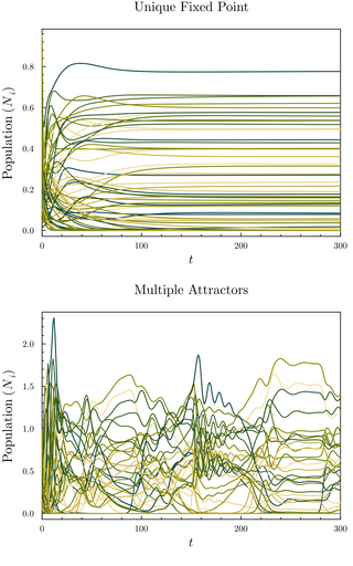
In theoretical ecology and nonlinear dynamics, consumer-resource models (CRMs) are a class of ecological models in which a community of consumer species compete for a common pool of resources. Instead of species interacting directly, all species-species interactions are mediated through resource dynamics. Consumer-resource models have served as fundamental tools in the quantitative development of theories of niche construction, coexistence, and biological diversity. These models can be interpreted as a quantitative description of a single trophic level.
The random generalized Lotka–Volterra model (rGLV) is an ecological model and random set of coupled ordinary differential equations where the parameters of the generalized Lotka–Volterra equation are sampled from a probability distribution, analogously to quenched disorder. The rGLV models dynamics of a community of species in which each species' abundance grows towards a carrying capacity but is depleted due to competition from the presence of other species. It is often analyzed in the many-species limit using tools from statistical physics, in particular from spin glass theory.
1 2 3 Bonsall, Michael B.; Hassell, Michael P. (2007). "Predator–prey interactions". In May, Robert; McLean, Angela (eds.). Theoretical Ecology: Principles and Applications (3rded.). Oxford University Press. pp.46–61.
↑ John D. Reeve; Wiliam W. Murdoch (1986). "Biological Control by the Parasitoid Aphytis melinus, and Population Stability of the California Red Scale". Journal of Animal Ecology. 55 (3): 1069–1082. Bibcode:1986JAnEc..55.1069R. doi:10.2307/4434. JSTOR4434.
↑ Grenfell, Bryan; Keeling, Matthew (2007). "Dynamics of infectious disease". In May, Robert; McLean, Angela (eds.). Theoretical Ecology: Principles and Applications (3rded.). Oxford University Press. pp.132–147.
↑ Takeuchi, Y. (1989). "Cooperative systems theory and global stability of diffusion models". Acta Applicandae Mathematicae. 14 (1–2): 49–57. doi:10.1007/BF00046673. S2CID189902519.
↑ This applies to British and American academics; landscape ecology has a distinct genesis among European academics.
↑ First introduced in MacArthur & Wilson's (1967) book of notable mention in the history and theoretical science of ecology, The Theory of Island Biogeography
↑ Thorp, J. H., & Delong, M. D. (1994). The Riverine Productivity Model: An Heuristic View of Carbon Sources and Organic Processing in Large River Ecosystems. Oikos, 305-308
↑ Benke, A. C., Chaubey, I., Ward, G. M., & Dunn, E. L. (2000). Flood Pulse Dynamics of an Unregulated River Floodplain in the Southeastern U.S. Coastal Plain. Ecology, 2730-2741.
The classic text is Theoretical Ecology: Principles and Applications, by Angela McLean and Robert May. The 2007 edition is published by the Oxford University Press. ISBN978-0-19-920998-9.
This page is based on this Wikipedia article Text is available under the CC BY-SA 4.0 license; additional terms may apply. Images, videos and audio are available under their respective licenses.