Ekman layer

Last updated
The Ekman layer is the layer in a fluid where the flow is the result of a balance between pressure gradient, Coriolis and turbulent drag forces. In the picture above, the wind blowing North creates a surface stress and a resulting Ekman spiral is found below it in the column of water. Ekman layer.jpg
The Ekman layer is the layer in a fluid where the flow is the result of a balance between pressure gradient, Coriolis and turbulent drag forces. In the picture above, the wind blowing North creates a surface stress and a resulting Ekman spiral is found below it in the column of water.

The Ekman layer is the layer in a fluid where there is a force balance between pressure gradient force, Coriolis force and turbulent drag. It was first described by Vagn Walfrid Ekman. Ekman layers occur both in the atmosphere and in the ocean.

Contents

There are two types of Ekman layers. The first type occurs at the surface of the ocean and is forced by surface winds, which act as a drag on the surface of the ocean. The second type occurs at the bottom of the atmosphere and ocean, where frictional forces are associated with flow over rough surfaces.

History

Ekman developed the theory of the Ekman layer after Fridtjof Nansen observed that ice drifts at an angle of 20°–40° to the right of the prevailing wind direction while on an Arctic expedition aboard the Fram. Nansen asked his colleague, Vilhelm Bjerknes to set one of his students upon study of the problem. Bjerknes tapped Ekman, who presented his results in 1902 as his doctoral thesis. [1]

Mathematical formulation

The mathematical formulation of the Ekman layer begins by assuming a neutrally stratified fluid, a balance between the forces of pressure gradient, Coriolis and turbulent drag.

where and are the velocities in the and directions, respectively, is the local Coriolis parameter, and is the diffusive eddy viscosity, which can be derived using mixing length theory. Note that is a modified pressure: we have incorporated the hydrostatic of the pressure, to take account of gravity.

There are many regions where an Ekman layer is theoretically plausible; they include the bottom of the atmosphere, near the surface of the earth and ocean, the bottom of the ocean, near the sea floor and at the top of the ocean, near the air-water interface. Different boundary conditions are appropriate for each of these different situations. Each of these situations can be accounted for through the boundary conditions applied to the resulting system of ordinary differential equations. The separate cases of top and bottom boundary layers are shown below.

Ekman layer at the ocean (or free) surface

We will consider boundary conditions of the Ekman layer in the upper ocean: [2]

where and are the components of the surface stress, , of the wind field or ice layer at the top of the ocean, and is the dynamic viscosity.

For the boundary condition on the other side, as , where and are the geostrophic flows in the and directions.

Solution

Three views of the wind-driven Ekman layer at the surface of the ocean in the Northern Hemisphere. The geostrophic velocity is zero in this example. EkmanSpiral.svg
Three views of the wind-driven Ekman layer at the surface of the ocean in the Northern Hemisphere. The geostrophic velocity is zero in this example.

These differential equations can be solved to find:

The value is called the Ekman layer depth, and gives an indication of the penetration depth of wind-induced turbulent mixing in the ocean. Note that it varies on two parameters: the turbulent diffusivity , and the latitude, as encapsulated by . For a typical m/s, and at 45° latitude ( s), then is approximately 45 meters. This Ekman depth prediction does not always agree precisely with observations.

This variation of horizontal velocity with depth () is referred to as the Ekman spiral, diagrammed above and at right.

By applying the continuity equation we can have the vertical velocity as following

Note that when vertically-integrated, the volume transport associated with the Ekman spiral is to the right of the wind direction in the Northern Hemisphere.

Ekman layer at the bottom of the ocean and atmosphere

The traditional development of Ekman layers bounded below by a surface utilizes two boundary conditions:

Experimental observations of the Ekman layer

There is much difficulty associated with observing the Ekman layer for two main reasons: the theory is too simplistic as it assumes a constant eddy viscosity, which Ekman himself anticipated, [3] saying

It is obvious that cannot generally be regarded as a constant when the density of water is not uniform within the region considered

and because it is difficult to design instruments with great enough sensitivity to observe the velocity profile in the ocean.

Laboratory demonstrations

The bottom Ekman layer can readily be observed in a rotating cylindrical tank of water by dropping in dye and changing the rotation rate slightly. Archived 2013-10-22 at the Wayback Machine Surface Ekman layers can also be observed in rotating tanks.

In the atmosphere

In the atmosphere, the Ekman solution generally overstates the magnitude of the horizontal wind field because it does not account for the velocity shear in the surface layer. Splitting the planetary boundary layer into the surface layer and the Ekman layer generally yields more accurate results. [4]

In the ocean

The Ekman layer, with its distinguishing feature the Ekman spiral, is rarely observed in the ocean. The Ekman layer near the surface of the ocean extends only about 10 – 20 meters deep, [4] and instrumentation sensitive enough to observe a velocity profile in such a shallow depth has only been available since around 1980. [2] Also, wind waves modify the flow near the surface, and make observations close to the surface rather difficult. [5]

Instrumentation

Observations of the Ekman layer have only been possible since the development of robust surface moorings and sensitive current meters. Ekman himself developed a current meter to observe the spiral that bears his name, but was not successful. [6] The Vector Measuring Current Meter [7] and the Acoustic Doppler Current Profiler are both used to measure current.

Observations

The first documented observations of an Ekman-like spiral in the ocean were made in the Arctic Ocean from a drifting ice floe in 1958. [8] More recent observations include (not an exhaustive list):

  • The 1980 mixed layer experiment [9]
  • Within the Sargasso Sea during the 1982 Long Term Upper Ocean Study [10]
  • Within the California Current during the 1993 Eastern Boundary Current experiment [11]
  • Within the Drake Passage region of the Southern Ocean [12]
  • In the eastern tropical Pacific, at 2°N, 140°W, using 5 current meters between 5 and 25 meters depth. [13] This study noted that the geostrophic shear associated with tropical stability waves modified the Ekman spiral relative to what is expected with horizontally uniform density.
  • North of the Kerguelen Plateau during the 2008 SOFINE experiment [14]

Common to several of these observations spirals were found to be "compressed", displaying larger estimates of eddy viscosity when considering the rate of rotation with depth than the eddy viscosity derived from considering the rate of decay of speed. [10] [11] [12] [14]

See also

Related Research Articles

<span class="mw-page-title-main">Navier–Stokes equations</span> Equations describing the motion of viscous fluid substances

The Navier–Stokes equations are partial differential equations which describe the motion of viscous fluid substances. They were named after French engineer and physicist Claude-Louis Navier and the Irish physicist and mathematician George Gabriel Stokes. They were developed over several decades of progressively building the theories, from 1822 (Navier) to 1842–1850 (Stokes).

<span class="mw-page-title-main">Potential flow</span> Velocity field as the gradient of a scalar function

In fluid dynamics, potential flow is the ideal flow pattern of an inviscid fluid. Potential flows are described and determined by mathematical methods.

The vorticity equation of fluid dynamics describes the evolution of the vorticity ω of a particle of a fluid as it moves with its flow; that is, the local rotation of the fluid. The governing equation is:

<span class="mw-page-title-main">Boundary layer</span> Layer of fluid in the immediate vicinity of a bounding surface

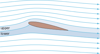
In physics and fluid mechanics, a boundary layer is the thin layer of fluid in the immediate vicinity of a bounding surface formed by the fluid flowing along the surface. The fluid's interaction with the wall induces a no-slip boundary condition. The flow velocity then monotonically increases above the surface until it returns to the bulk flow velocity. The thin layer consisting of fluid whose velocity has not yet returned to the bulk flow velocity is called the velocity boundary layer.

In atmospheric science, geostrophic flow is the theoretical wind that would result from an exact balance between the Coriolis force and the pressure gradient force. This condition is called geostrophic equilibrium or geostrophic balance. The geostrophic wind is directed parallel to isobars. This balance seldom holds exactly in nature. The true wind almost always differs from the geostrophic wind due to other forces such as friction from the ground. Thus, the actual wind would equal the geostrophic wind only if there were no friction and the isobars were perfectly straight. Despite this, much of the atmosphere outside the tropics is close to geostrophic flow much of the time and it is a valuable first approximation. Geostrophic flow in air or water is a zero-frequency inertial wave.

<span class="mw-page-title-main">Ekman spiral</span> Velocity profile of wind driven current with depth

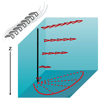
The Ekman spiral is an arrangement of ocean currents: the directions of horizontal current appear to twist as the depth changes. The oceanic wind driven Ekman spiral is the result of a force balance created by a shear stress force, Coriolis force and the water drag. This force balance gives a resulting current of the water different from the winds. In the ocean, there are two places where the Ekman spiral can be observed. At the surface of the ocean, the shear stress force corresponds with the wind stress force. At the bottom of the ocean, the shear stress force is created by friction with the ocean floor. This phenomenon was first observed at the surface by the Norwegian oceanographer Fridtjof Nansen during his Fram expedition. He noticed that icebergs did not drift in the same direction as the wind. His student, the Swedish oceanographer Vagn Walfrid Ekman, was the first person to physically explain this process.

The Sverdrup balance, or Sverdrup relation, is a theoretical relationship between the wind stress exerted on the surface of the open ocean and the vertically integrated meridional (north-south) transport of ocean water.

In physics and fluid mechanics, a Blasius boundary layer describes the steady two-dimensional laminar boundary layer that forms on a semi-infinite plate which is held parallel to a constant unidirectional flow. Falkner and Skan later generalized Blasius' solution to wedge flow, i.e. flows in which the plate is not parallel to the flow.

<span class="mw-page-title-main">Ekman transport</span> Net transport of surface water perpendicular to wind direction

Ekman transport is part of Ekman motion theory, first investigated in 1902 by Vagn Walfrid Ekman. Winds are the main source of energy for ocean circulation, and Ekman transport is a component of wind-driven ocean current. Ekman transport occurs when ocean surface waters are influenced by the friction force acting on them via the wind. As the wind blows it casts a friction force on the ocean surface that drags the upper 10-100m of the water column with it. However, due to the influence of the Coriolis effect, the ocean water moves at a 90° angle from the direction of the surface wind. The direction of transport is dependent on the hemisphere: in the northern hemisphere, transport occurs at 90° clockwise from wind direction, while in the southern hemisphere it occurs at 90° anticlockwise. This phenomenon was first noted by Fridtjof Nansen, who recorded that ice transport appeared to occur at an angle to the wind direction during his Arctic expedition of the 1890s. Ekman transport has significant impacts on the biogeochemical properties of the world's oceans. This is because it leads to upwelling and downwelling in order to obey mass conservation laws. Mass conservation, in reference to Ekman transfer, requires that any water displaced within an area must be replenished. This can be done by either Ekman suction or Ekman pumping depending on wind patterns.

The derivation of the Navier–Stokes equations as well as its application and formulation for different families of fluids, is an important exercise in fluid dynamics with applications in mechanical engineering, physics, chemistry, heat transfer, and electrical engineering. A proof explaining the properties and bounds of the equations, such as Navier–Stokes existence and smoothness, is one of the important unsolved problems in mathematics.

The Cebeci–Smith model, developed by Tuncer Cebeci and Apollo M. O. Smith in 1967, is a 0-equation eddy viscosity model used in computational fluid dynamics analysis of turbulence in boundary layer flows. The model gives eddy viscosity, , as a function of the local boundary layer velocity profile. The model is suitable for high-speed flows with thin attached boundary layers, typically present in aerospace applications. Like the Baldwin-Lomax model, it is not suitable for large regions of flow separation and significant curvature or rotation. Unlike the Baldwin-Lomax model, this model requires the determination of a boundary layer edge.

In physical oceanography and fluid dynamics, the wind stress is the shear stress exerted by the wind on the surface of large bodies of water – such as oceans, seas, estuaries and lakes. When wind is blowing over a water surface, the wind applies a wind force on the water surface. The wind stress is the component of this wind force that is parallel to the surface per unit area. Also, the wind stress can be described as the flux of horizontal momentum applied by the wind on the water surface. The wind stress causes a deformation of the water body whereby wind waves are generated. Also, the wind stress drives ocean currents and is therefore an important driver of the large-scale ocean circulation. The wind stress is affected by the wind speed, the shape of the wind waves and the atmospheric stratification. It is one of the components of the air–sea interaction, with others being the atmospheric pressure on the water surface, as well as the exchange of energy and mass between the water and the atmosphere.

The Cauchy momentum equation is a vector partial differential equation put forth by Cauchy that describes the non-relativistic momentum transport in any continuum.

Shear velocity, also called friction velocity, is a form by which a shear stress may be re-written in units of velocity. It is useful as a method in fluid mechanics to compare true velocities, such as the velocity of a flow in a stream, to a velocity that relates shear between layers of flow.

In fluid dynamics, Airy wave theory gives a linearised description of the propagation of gravity waves on the surface of a homogeneous fluid layer. The theory assumes that the fluid layer has a uniform mean depth, and that the fluid flow is inviscid, incompressible and irrotational. This theory was first published, in correct form, by George Biddell Airy in the 19th century.

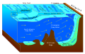
Ocean dynamics define and describe the flow of water within the oceans. Ocean temperature and motion fields can be separated into three distinct layers: mixed (surface) layer, upper ocean, and deep ocean.

<span class="mw-page-title-main">Radiation stress</span> Term in physical oceanography

In fluid dynamics, the radiation stress is the depth-integrated – and thereafter phase-averaged – excess momentum flux caused by the presence of the surface gravity waves, which is exerted on the mean flow. The radiation stresses behave as a second-order tensor.

In oceanography, Ekman velocity – also referred as a kind of the residual ageostrophic velocity as it deviates from geostrophy – is part of the total horizontal velocity (u) in the upper layer of water of the open ocean. This velocity, caused by winds blowing over the surface of the ocean, is such that the Coriolis force on this layer is balanced by the force of the wind.

In physical oceanography and fluid mechanics, the Miles-Phillips mechanism describes the generation of wind waves from a flat sea surface by two distinct mechanisms. Wind blowing over the surface generates tiny wavelets. These wavelets develop over time and become ocean surface waves by absorbing the energy transferred from the wind. The Miles-Phillips mechanism is a physical interpretation of these wind-generated surface waves.
Both mechanisms are applied to gravity-capillary waves and have in common that waves are generated by a resonance phenomenon. The Miles mechanism is based on the hypothesis that waves arise as an instability of the sea-atmosphere system. The Phillips mechanism assumes that turbulent eddies in the atmospheric boundary layer induce pressure fluctuations at the sea surface. The Phillips mechanism is generally assumed to be important in the first stages of wave growth, whereas the Miles mechanism is important in later stages where the wave growth becomes exponential in time.

The recharge oscillator model for El Niño–Southern Oscillation (ENSO) is a theory described for the first time in 1997 by Jin., which explains the periodical variation of the sea surface temperature (SST) and thermocline depth that occurs in the central equatorial Pacific Ocean. The physical mechanisms at the basis of this oscillation are periodical recharges and discharges of the zonal mean equatorial heat content, due to ocean-atmosphere interaction. Other theories have been proposed to model ENSO, such as the delayed oscillator, the western Pacific oscillator and the advective reflective oscillator. A unified and consistent model has been proposed by Wang in 2001, in which the recharge oscillator model is included as a particular case.

References

  1. Cushman-Roisin, Benoit (1994). "Chapter 5 – The Ekman Layer". Introduction to Geophysical Fluid Dynamics (1st ed.). Prentice Hall. pp. 76–77. ISBN   978-0-13-353301-9.
  2. 1 2 Vallis, Geoffrey K. (2006). "Chapter 2 – Effects of Rotation and Stratification". Atmospheric and Oceanic Fluid Dynamics (1st ed.). Cambridge, UK: Cambridge University Press. pp. 112–113. ISBN   978-0-521-84969-2.
  3. Ekman, V.W. (1905). "On the influence of the earth's rotation on ocean currents". Ark. Mat. Astron. Fys. 2 (11): 1–52.
  4. 1 2 Holton, James R. (2004). "Chapter 5 – The Planetary Boundary Layer". Dynamic Meteorology. International Geophysics Series. Vol. 88 (4th ed.). Burlington, MA: Elsevier Academic Press. pp. 129–130. ISBN   978-0-12-354015-7.
  5. Santala, M. J.; Terray, E. A. (1992). "A technique for making unbiased estimates of current shear from a wave-follower". Deep-Sea Research. 39 (3–4): 607–622. Bibcode:1992DSRA...39..607S. doi:10.1016/0198-0149(92)90091-7.
  6. Rudnick, Daniel (2003). "Observations of Momentum Transfer in the Upper Ocean: Did Ekman Get It Right?". Near-Boundary Processes and Their Parameterization. Manoa, Hawaii: School of Ocean and Earth Science and Technology.
  7. Weller, R.A.; Davis, R.E. (1980). "A vector-measuring current meter". Deep-Sea Research. 27 (7): 565–582. Bibcode:1980DSRA...27..565W. doi:10.1016/0198-0149(80)90041-2.
  8. Hunkins, K. (1966). "Ekman drift currents in the Arctic Ocean". Deep-Sea Research. 13 (4): 607–620. Bibcode:1966DSRA...13..607H. doi:10.1016/0011-7471(66)90592-4.
  9. Davis, R.E.; de Szoeke, R.; Niiler., P. (1981). "Part II: Modelling the mixed layer response". Deep-Sea Research. 28 (12): 1453–1475. Bibcode:1981DSRA...28.1453D. doi:10.1016/0198-0149(81)90092-3.
  10. 1 2 Price, J.F.; Weller, R.A.; Schudlich, R.R. (1987). "Wind-Driven Ocean Currents and Ekman Transport". Science. 238 (4833): 1534–1538. Bibcode:1987Sci...238.1534P. doi:10.1126/science.238.4833.1534. PMID   17784291. S2CID   45511024.
  11. 1 2 Chereskin, T.K. (1995). "Direct evidence for an Ekman balance in the California Current". Journal of Geophysical Research. 100 (C9): 18261–18269. Bibcode:1995JGR...10018261C. doi:10.1029/95JC02182.
  12. 1 2 Lenn, Y; Chereskin, T.K. (2009). "Observation of Ekman Currents in the Southern Ocean". Journal of Physical Oceanography. 39 (3): 768–779. Bibcode:2009JPO....39..768L. doi: 10.1175/2008jpo3943.1 . S2CID   129107187.
  13. Cronin, M.F.; Kessler, W.S. (2009). "Near-Surface Shear Flow in the Tropical Pacific Cold Tongue Front". Journal of Physical Oceanography. 39 (5): 1200–1215. Bibcode:2009JPO....39.1200C. CiteSeerX   10.1.1.517.8028 . doi:10.1175/2008JPO4064.1.
  14. 1 2 Roach, C.J.; Phillips, H.E.; Bindoff, N.L.; Rintoul, S.R. (2015). "Detecting and Characterizing Ekman Currents in the Southern Ocean". Journal of Physical Oceanography. 45 (5): 1205–1223. Bibcode:2015JPO....45.1205R. doi: 10.1175/JPO-D-14-0115.1 .