Boussinesq approximation (water waves)

Last updated
Simulation of periodic waves over an underwater shoal with a Boussinesq-type model. The waves propagate over an elliptic-shaped underwater shoal on a plane beach. This example combines several effects of waves and shallow water, including refraction, diffraction, shoaling and weak non-linearity. Bous2d berk03 z.gif
Simulation of periodic waves over an underwater shoal with a Boussinesq-type model. The waves propagate over an elliptic-shaped underwater shoal on a plane beach. This example combines several effects of waves and shallow water, including refraction, diffraction, shoaling and weak non-linearity.

In fluid dynamics, the Boussinesq approximation for water waves is an approximation valid for weakly non-linear and fairly long waves. The approximation is named after Joseph Boussinesq, who first derived them in response to the observation by John Scott Russell of the wave of translation (also known as solitary wave or soliton). The 1872 paper of Boussinesq introduces the equations now known as the Boussinesq equations. [1]

Contents

The Boussinesq approximation for water waves takes into account the vertical structure of the horizontal and vertical flow velocity. This results in non-linear partial differential equations, called Boussinesq-type equations, which incorporate frequency dispersion (as opposite to the shallow water equations, which are not frequency-dispersive). In coastal engineering, Boussinesq-type equations are frequently used in computer models for the simulation of water waves in shallow seas and harbours.

While the Boussinesq approximation is applicable to fairly long waves – that is, when the wavelength is large compared to the water depth – the Stokes expansion is more appropriate for short waves (when the wavelength is of the same order as the water depth, or shorter).

Boussinesq approximation

Periodic waves in the Boussinesq approximation, shown in a vertical cross section in the wave propagation direction. Notice the flat troughs and sharp crests, due to the wave nonlinearity. This case (drawn on scale) shows a wave with the wavelength equal to 39.1 m, the wave height is 1.8 m (i.e. the difference between crest and trough elevation), and the mean water depth is 5 m, while the gravitational acceleration is 9.81 m/s . Boussinesq T06H18d5.svg
Periodic waves in the Boussinesq approximation, shown in a vertical cross section in the wave propagation direction. Notice the flat troughs and sharp crests, due to the wave nonlinearity. This case (drawn on scale) shows a wave with the wavelength equal to 39.1  m, the wave height is 1.8 m (i.e. the difference between crest and trough elevation), and the mean water depth is 5 m, while the gravitational acceleration is 9.81 m/s .

The essential idea in the Boussinesq approximation is the elimination of the vertical coordinate from the flow equations, while retaining some of the influences of the vertical structure of the flow under water waves. This is useful because the waves propagate in the horizontal plane and have a different (not wave-like) behaviour in the vertical direction. Often, as in Boussinesq's case, the interest is primarily in the wave propagation.

This elimination of the vertical coordinate was first done by Joseph Boussinesq in 1871, to construct an approximate solution for the solitary wave (or wave of translation). Subsequently, in 1872, Boussinesq derived the equations known nowadays as the Boussinesq equations.

The steps in the Boussinesq approximation are:

Thereafter, the Boussinesq approximation is applied to the remaining flow equations, in order to eliminate the dependence on the vertical coordinate. As a result, the resulting partial differential equations are in terms of functions of the horizontal coordinates (and time).

As an example, consider potential flow over a horizontal bed in the plane, with the horizontal and the vertical coordinate. The bed is located at , where is the mean water depth. A Taylor expansion is made of the velocity potential around the bed level : [2]

where is the velocity potential at the bed. Invoking Laplace's equation for , as valid for incompressible flow, gives:

since the vertical velocity is zero at the – impermeable – horizontal bed . This series may subsequently be truncated to a finite number of terms.

Original Boussinesq equations

Derivation

For water waves on an incompressible fluid and irrotational flow in the plane, the boundary conditions at the free surface elevation are: [3]

where:

Now the Boussinesq approximation for the velocity potential , as given above, is applied in these boundary conditions. Further, in the resulting equations only the linear and quadratic terms with respect to and are retained (with the horizontal velocity at the bed ). The cubic and higher order terms are assumed to be negligible. Then, the following partial differential equations are obtained:

set A – Boussinesq (1872), equation (25)

This set of equations has been derived for a flat horizontal bed, i.e. the mean depth is a constant independent of position . When the right-hand sides of the above equations are set to zero, they reduce to the shallow water equations.

Under some additional approximations, but at the same order of accuracy, the above set A can be reduced to a single partial differential equation for the free surface elevation :

set B – Boussinesq (1872), equation (26)

From the terms between brackets, the importance of nonlinearity of the equation can be expressed in terms of the Ursell number. In dimensionless quantities, using the water depth and gravitational acceleration for non-dimensionalization, this equation reads, after normalization: [4]

with:

: the dimensionless surface elevation,
: the dimensionless time, and
: the dimensionless horizontal position.
Linear phase speed squared
c
2
/
(
g
h
)
{\displaystyle c^{2}/(gh)}
as a function of relative wave number
k
h
{\displaystyle kh}
.
A = Boussinesq (1872), equation (25),
B = Boussinesq (1872), equation (26),
C = full linear wave theory, see dispersion (water waves) Disp bouss.svg
Linear phase speed squared as a function of relative wave number .
A = Boussinesq (1872), equation (25),
B = Boussinesq (1872), equation (26),
C = full linear wave theory, see dispersion (water waves)

Linear frequency dispersion

Water waves of different wave lengths travel with different phase speeds, a phenomenon known as frequency dispersion. For the case of infinitesimal wave amplitude, the terminology is linear frequency dispersion. The frequency dispersion characteristics of a Boussinesq-type of equation can be used to determine the range of wave lengths, for which it is a valid approximation.

The linear frequency dispersion characteristics for the above set A of equations are: [5]

with:

The relative error in the phase speed for set A, as compared with linear theory for water waves, is less than 4% for a relative wave number . So, in engineering applications, set A is valid for wavelengths larger than 4 times the water depth .

The linear frequency dispersion characteristics of equation B are: [5]

The relative error in the phase speed for equation B is less than 4% for , equivalent to wave lengths longer than 7 times the water depth , called fairly long waves. [6]

For short waves with equation B become physically meaningless, because there are no longer real-valued solutions of the phase speed. The original set of two partial differential equations (Boussinesq, 1872, equation 25, see set A above) does not have this shortcoming.

The shallow water equations have a relative error in the phase speed less than 4% for wave lengths in excess of 13 times the water depth .

Boussinesq-type equations and extensions

There are an overwhelming number of mathematical models which are referred to as Boussinesq equations. This may easily lead to confusion, since often they are loosely referenced to as the Boussinesq equations, while in fact a variant thereof is considered. So it is more appropriate to call them Boussinesq-type equations. Strictly speaking, the Boussinesq equations is the above-mentioned set B, since it is used in the analysis in the remainder of his 1872 paper.

Some directions, into which the Boussinesq equations have been extended, are:

Further approximations for one-way wave propagation

While the Boussinesq equations allow for waves traveling simultaneously in opposing directions, it is often advantageous to only consider waves traveling in one direction. Under small additional assumptions, the Boussinesq equations reduce to:

Besides solitary wave solutions, the Korteweg–de Vries equation also has periodic and exact solutions, called cnoidal waves. These are approximate solutions of the Boussinesq equation.

Numerical models

A simulation with a Boussinesq-type wave model of nearshore waves travelling towards a harbour entrance. The simulation is with the BOUSS-2D module of SMS. Bouss-2D simulation of nearshore waves.jpg
A simulation with a Boussinesq-type wave model of nearshore waves travelling towards a harbour entrance. The simulation is with the BOUSS-2D module of SMS.
Faster than real-time simulation with the Boussinesq module of Celeris, showing wave breaking and refraction near the beach. The model provides an interactive environment. Celeris Wave Model.gif
Faster than real-time simulation with the Boussinesq module of Celeris, showing wave breaking and refraction near the beach. The model provides an interactive environment.

For the simulation of wave motion near coasts and harbours, numerical models – both commercial and academic – employing Boussinesq-type equations exist. Some commercial examples are the Boussinesq-type wave modules in MIKE 21 and SMS. Some of the free Boussinesq models are Celeris, [7] COULWAVE, [8] and FUNWAVE. [9] Most numerical models employ finite-difference, finite-volume or finite element techniques for the discretization of the model equations. Scientific reviews and intercomparisons of several Boussinesq-type equations, their numerical approximation and performance are e.g. Kirby (2003), Dingemans (1997 , Part 2, Chapter 5) and Hamm, Madsen & Peregrine (1993).

Notes

  1. This paper (Boussinesq, 1872) starts with: "Tous les ingénieurs connaissent les belles expériences de J. Scott Russell et M. Basin sur la production et la propagation des ondes solitaires" ("All engineers know the beautiful experiments of J. Scott Russell and M. Basin on the generation and propagation of solitary waves").
  2. Dingemans (1997), p. 477.
  3. Dingemans (1997), p. 475.
  4. Johnson (1997), p. 219
  5. 1 2 Dingemans (1997), p. 521.
  6. Dingemans (1997), p. 473 & 516.
  7. "Celeria.org - Celeris Boussinesq Wave Model". Celeria.org - Celeris Boussinesq Wave Model.
  8. "ISEC - Models". isec.nacse.org.
  9. "James T. Kirby, Funwave program". www1.udel.edu.

Related Research Articles

<span class="mw-page-title-main">Dirac delta function</span> Generalized function whose value is zero everywhere except at zero

In mathematics, the Dirac delta distribution, also known as the unit impulse, is a generalized function or distribution over the real numbers, whose value is zero everywhere except at zero, and whose integral over the entire real line is equal to one.

<span class="mw-page-title-main">Navier–Stokes equations</span> Equations describing the motion of viscous fluid substances

In physics, the Navier–Stokes equations are partial differential equations which describe the motion of viscous fluid substances, named after French engineer and physicist Claude-Louis Navier and Anglo-Irish physicist and mathematician George Gabriel Stokes. They were developed over several decades of progressively building the theories, from 1822 (Navier) to 1842–1850 (Stokes).

<span class="mw-page-title-main">Potential flow</span> Velocity field as the gradient of a scalar function

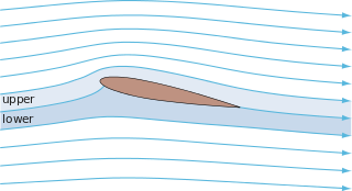
In fluid dynamics, potential flow describes the velocity field as the gradient of a scalar function: the velocity potential. As a result, a potential flow is characterized by an irrotational velocity field, which is a valid approximation for several applications. The irrotationality of a potential flow is due to the curl of the gradient of a scalar always being equal to zero.

<span class="mw-page-title-main">Gravity wave</span> Wave in or at the interface between fluids where gravity is the main equilibrium force

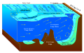
In fluid dynamics, gravity waves are waves generated in a fluid medium or at the interface between two media when the force of gravity or buoyancy tries to restore equilibrium. An example of such an interface is that between the atmosphere and the ocean, which gives rise to wind waves.

The primitive equations are a set of nonlinear partial differential equations that are used to approximate global atmospheric flow and are used in most atmospheric models. They consist of three main sets of balance equations:

  1. A continuity equation: Representing the conservation of mass.
  2. Conservation of momentum: Consisting of a form of the Navier–Stokes equations that describe hydrodynamical flow on the surface of a sphere under the assumption that vertical motion is much smaller than horizontal motion (hydrostasis) and that the fluid layer depth is small compared to the radius of the sphere
  3. A thermal energy equation: Relating the overall temperature of the system to heat sources and sinks

In physics and fluid mechanics, a Blasius boundary layer describes the steady two-dimensional laminar boundary layer that forms on a semi-infinite plate which is held parallel to a constant unidirectional flow. Falkner and Skan later generalized Blasius' solution to wedge flow, i.e. flows in which the plate is not parallel to the flow.

<span class="mw-page-title-main">Shallow water equations</span> Set of partial differential equations that describe the flow below a pressure surface in a fluid

The shallow-water equations (SWE) are a set of hyperbolic partial differential equations that describe the flow below a pressure surface in a fluid. The shallow-water equations in unidirectional form are also called Saint-Venant equations, after Adhémar Jean Claude Barré de Saint-Venant.

Atmospheric tides are global-scale periodic oscillations of the atmosphere. In many ways they are analogous to ocean tides. Atmospheric tides can be excited by:

<span class="mw-page-title-main">Stokes drift</span> Average velocity of a fluid parcel in a gravity wave

For a pure wave motion in fluid dynamics, the Stokes drift velocity is the average velocity when following a specific fluid parcel as it travels with the fluid flow. For instance, a particle floating at the free surface of water waves, experiences a net Stokes drift velocity in the direction of wave propagation.

<span class="mw-page-title-main">Stokes wave</span> Nonlinear and periodic surface wave on an inviscid fluid layer of constant mean depth

In fluid dynamics, a Stokes wave is a nonlinear and periodic surface wave on an inviscid fluid layer of constant mean depth. This type of modelling has its origins in the mid 19th century when Sir George Stokes – using a perturbation series approach, now known as the Stokes expansion – obtained approximate solutions for nonlinear wave motion.

The omega equation is a culminating result in synoptic-scale meteorology. It is an elliptic partial differential equation, named because its left-hand side produces an estimate of vertical velocity, customarily expressed by symbol , in a pressure coordinate measuring height the atmosphere. Mathematically, , where represents a material derivative. The underlying concept is more general, however, and can also be applied to the Boussinesq fluid equation system where vertical velocity is in altitude coordinate z.

In fluid dynamics, Luke's variational principle is a Lagrangian variational description of the motion of surface waves on a fluid with a free surface, under the action of gravity. This principle is named after J.C. Luke, who published it in 1967. This variational principle is for incompressible and inviscid potential flows, and is used to derive approximate wave models like the mild-slope equation, or using the averaged Lagrangian approach for wave propagation in inhomogeneous media.

In fluid dynamics, Airy wave theory gives a linearised description of the propagation of gravity waves on the surface of a homogeneous fluid layer. The theory assumes that the fluid layer has a uniform mean depth, and that the fluid flow is inviscid, incompressible and irrotational. This theory was first published, in correct form, by George Biddell Airy in the 19th century.

<span class="mw-page-title-main">Mild-slope equation</span> Physics phenomenon and formula

In fluid dynamics, the mild-slope equation describes the combined effects of diffraction and refraction for water waves propagating over bathymetry and due to lateral boundaries—like breakwaters and coastlines. It is an approximate model, deriving its name from being originally developed for wave propagation over mild slopes of the sea floor. The mild-slope equation is often used in coastal engineering to compute the wave-field changes near harbours and coasts.

Equatorial Rossby waves, often called planetary waves, are very long, low frequency water waves found near the equator and are derived using the equatorial beta plane approximation.

<span class="mw-page-title-main">Cnoidal wave</span> Nonlinear and exact periodic wave solution of the Korteweg–de Vries equation

In fluid dynamics, a cnoidal wave is a nonlinear and exact periodic wave solution of the Korteweg–de Vries equation. These solutions are in terms of the Jacobi elliptic function cn, which is why they are coined cnoidal waves. They are used to describe surface gravity waves of fairly long wavelength, as compared to the water depth.

<span class="mw-page-title-main">Radiation stress</span> Term in physical oceanography

In fluid dynamics, the radiation stress is the depth-integrated – and thereafter phase-averaged – excess momentum flux caused by the presence of the surface gravity waves, which is exerted on the mean flow. The radiation stresses behave as a second-order tensor.

<span class="mw-page-title-main">Green's law</span> Equation describing evolution of waves in shallow water

In fluid dynamics, Green's law, named for 19th-century British mathematician George Green, is a conservation law describing the evolution of non-breaking, surface gravity waves propagating in shallow water of gradually varying depth and width. In its simplest form, for wavefronts and depth contours parallel to each other, it states:

The Sack–Schamel equation describes the nonlinear evolution of the cold ion fluid in a two-component plasma under the influence of a self-organized electric field. It is a partial differential equation of second order in time and space formulated in Lagrangian coordinates. The dynamics described by the equation take place on an ionic time scale, which allows electrons to be treated as if they were in equilibrium and described by an isothermal Boltzmann distribution. Supplemented by suitable boundary conditions, it describes the entire configuration space of possible events the ion fluid is capable of, both globally and locally.

Nonlinear tides are generated by hydrodynamic distortions of tides. A tidal wave is said to be nonlinear when its shape deviates from a pure sinusoidal wave. In mathematical terms, the wave owes its nonlinearity due to the nonlinear advection and frictional terms in the governing equations. These become more important in shallow-water regions such as in estuaries. Nonlinear tides are studied in the fields of coastal morphodynamics, coastal engineering and physical oceanography. The nonlinearity of tides has important implications for the transport of sediment.

References