Luke's Lagrangian
Luke's Lagrangian formulation is for non-linear surface gravity waves on an—incompressible, irrotational and inviscid—potential flow.
The relevant ingredients, needed in order to describe this flow, are:
- Φ(x,z,t) is the velocity potential,
- ρ is the fluid density,
- g is the acceleration by the Earth's gravity,
- x is the horizontal coordinate vector with components x and y,
- x and y are the horizontal coordinates,
- z is the vertical coordinate,
- t is time, and
- ∇ is the horizontal gradient operator, so ∇Φ is the horizontal flow velocity consisting of ∂Φ/∂x and ∂Φ/∂y,
- V(t) is the time-dependent fluid domain with free surface.
The Lagrangian  , as given by Luke, is:

From Bernoulli's principle, this Lagrangian can be seen to be the integral of the fluid pressure over the whole time-dependent fluid domain V(t). This is in agreement with the variational principles for inviscid flow without a free surface, found by Harry Bateman. [7]
Variation with respect to the velocity potential Φ(x,z,t) and free-moving surfaces like z = η(x,t) results in the Laplace equation for the potential in the fluid interior and all required boundary conditions: kinematic boundary conditions on all fluid boundaries and dynamic boundary conditions on free surfaces. [8] This may also include moving wavemaker walls and ship motion.
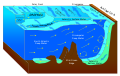
For the case of a horizontally unbounded domain with the free fluid surface at z = η(x,t) and a fixed bed at z = −h(x), Luke's variational principle results in the Lagrangian:

The bed-level term proportional to h2 in the potential energy has been neglected, since it is a constant and does not contribute in the variations. Below, Luke's variational principle is used to arrive at the flow equations for non-linear surface gravity waves on a potential flow.
Derivation of the flow equations resulting from Luke's variational principle
The variation  in the Lagrangian with respect to variations in the velocity potential Φ(x,z,t), as well as with respect to the surface elevation η(x,t), have to be zero. We consider both variations subsequently.
Variation with respect to the velocity potential
Consider a small variation δΦ in the velocity potential Φ. [8] Then the resulting variation in the Lagrangian is:

Using Leibniz integral rule, this becomes, in case of constant density ρ: [8]

The first integral on the right-hand side integrates out to the boundaries, in x and t, of the integration domain and is zero since the variations δΦ are taken to be zero at these boundaries. For variations δΦ which are zero at the free surface and the bed, the second integral remains, which is only zero for arbitrary δΦ in the fluid interior if there the Laplace equation holds:

with Δ = ∇ ⋅ ∇ + ∂2/∂z2 the Laplace operator.
If variations δΦ are considered which are only non-zero at the free surface, only the third integral remains, giving rise to the kinematic free-surface boundary condition:

Similarly, variations δΦ only non-zero at the bottom z = −h result in the kinematic bed condition:

Variation with respect to the surface elevation
Considering the variation of the Lagrangian with respect to small changes δη gives:

This has to be zero for arbitrary δη, giving rise to the dynamic boundary condition at the free surface:

This is the Bernoulli equation for unsteady potential flow, applied at the free surface, and with the pressure above the free surface being a constant — which constant pressure is taken equal to zero for simplicity.
The Hamiltonian structure of surface gravity waves on a potential flow was discovered by Vladimir E. Zakharov in 1968, and rediscovered independently by Bert Broer and John Miles: [4] [5] [6]

where the surface elevation η and surface potential φ — which is the potential Φ at the free surface z = η(x,t) — are the canonical variables. The Hamiltonian  is the sum of the kinetic and potential energy of the fluid:

The additional constraint is that the flow in the fluid domain has to satisfy Laplace's equation with appropriate boundary condition at the bottom z = −h(x) and that the potential at the free surface z = η is equal to φ: 
The Hamiltonian formulation can be derived from Luke's Lagrangian description by using Leibniz integral rule on the integral of ∂Φ/∂t: [6]

with  the value of the velocity potential at the free surface, and
  the Hamiltonian density — sum of the kinetic and potential energy density — and related to the Hamiltonian as:

The Hamiltonian density is written in terms of the surface potential using Green's third identity on the kinetic energy: [9]

where D(η) φ is equal to the normal derivative of ∂Φ/∂n at the free surface. Because of the linearity of the Laplace equation — valid in the fluid interior and depending on the boundary condition at the bed z = −h and free surface z = η — the normal derivative ∂Φ/∂n is a linear function of the surface potential φ, but depends non-linear on the surface elevation η. This is expressed by the Dirichlet-to-Neumann operator D(η), acting linearly on φ.
The Hamiltonian density can also be written as: [6]

with w(x,t) = ∂Φ/∂z the vertical velocity at the free surface z = η. Also w is a linear function of the surface potential φ through the Laplace equation, but w depends non-linear on the surface elevation η: [9]

with W operating linear on φ, but being non-linear in η. As a result, the Hamiltonian is a quadratic functional of the surface potential φ. Also the potential energy part of the Hamiltonian is quadratic. The source of non-linearity in surface gravity waves is through the kinetic energy depending non-linear on the free surface shape η. [9]
Further ∇φ is not to be mistaken for the horizontal velocity ∇Φ at the free surface:

Taking the variations of the Lagrangian  with respect to the canonical variables
  and
and  gives:
provided in the fluid interior Φ satisfies the Laplace equation, ΔΦ = 0, as well as the bottom boundary condition at z = −h and Φ = φ at the free surface.

The Navier–Stokes equations are partial differential equations which describe the motion of viscous fluid substances. They were named after French engineer and physicist Claude-Louis Navier and the Irish physicist and mathematician George Gabriel Stokes. They were developed over several decades of progressively building the theories, from 1822 (Navier) to 1842–1850 (Stokes).

The stress–energy tensor, sometimes called the stress–energy–momentum tensor or the energy–momentum tensor, is a tensor physical quantity that describes the density and flux of energy and momentum in spacetime, generalizing the stress tensor of Newtonian physics. It is an attribute of matter, radiation, and non-gravitational force fields. This density and flux of energy and momentum are the sources of the gravitational field in the Einstein field equations of general relativity, just as mass density is the source of such a field in Newtonian gravity.
The vorticity equation of fluid dynamics describes the evolution of the vorticity ω of a particle of a fluid as it moves with its flow; that is, the local rotation of the fluid. The governing equation is:
In physics, a Langevin equation is a stochastic differential equation describing how a system evolves when subjected to a combination of deterministic and fluctuating ("random") forces. The dependent variables in a Langevin equation typically are collective (macroscopic) variables changing only slowly in comparison to the other (microscopic) variables of the system. The fast (microscopic) variables are responsible for the stochastic nature of the Langevin equation. One application is to Brownian motion, which models the fluctuating motion of a small particle in a fluid.
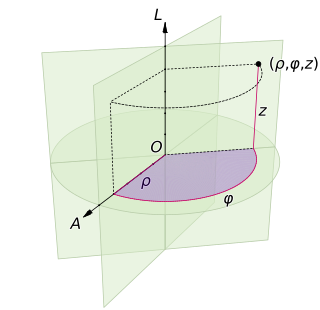
A cylindrical coordinate system is a three-dimensional coordinate system that specifies point positions by the distance from a chosen reference axis (axis L in the image opposite), the direction from the axis relative to a chosen reference direction (axis A), and the distance from a chosen reference plane perpendicular to the axis (plane containing the purple section). The latter distance is given as a positive or negative number depending on which side of the reference plane faces the point.
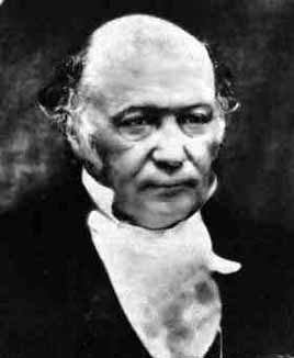
Hamiltonian mechanics emerged in 1833 as a reformulation of Lagrangian mechanics. Introduced by Sir William Rowan Hamilton, Hamiltonian mechanics replaces (generalized) velocities used in Lagrangian mechanics with (generalized) momenta. Both theories provide interpretations of classical mechanics and describe the same physical phenomena.
In the calculus of variations, a field of mathematical analysis, the functional derivative relates a change in a functional to a change in a function on which the functional depends.
This is a list of some vector calculus formulae for working with common curvilinear coordinate systems.
Hamiltonian fluid mechanics is the application of Hamiltonian methods to fluid mechanics. Note that this formalism only applies to nondissipative fluids.

The covariant formulation of classical electromagnetism refers to ways of writing the laws of classical electromagnetism in a form that is manifestly invariant under Lorentz transformations, in the formalism of special relativity using rectilinear inertial coordinate systems. These expressions both make it simple to prove that the laws of classical electromagnetism take the same form in any inertial coordinate system, and also provide a way to translate the fields and forces from one frame to another. However, this is not as general as Maxwell's equations in curved spacetime or non-rectilinear coordinate systems.
In theoretical physics, scalar field theory can refer to a relativistically invariant classical or quantum theory of scalar fields. A scalar field is invariant under any Lorentz transformation.
There are various mathematical descriptions of the electromagnetic field that are used in the study of electromagnetism, one of the four fundamental interactions of nature. In this article, several approaches are discussed, although the equations are in terms of electric and magnetic fields, potentials, and charges with currents, generally speaking.
The derivation of the Navier–Stokes equations as well as its application and formulation for different families of fluids, is an important exercise in fluid dynamics with applications in mechanical engineering, physics, chemistry, heat transfer, and electrical engineering. A proof explaining the properties and bounds of the equations, such as Navier–Stokes existence and smoothness, is one of the important unsolved problems in mathematics.
The Cauchy momentum equation is a vector partial differential equation put forth by Cauchy that describes the non-relativistic momentum transport in any continuum.
In fluid dynamics, Airy wave theory gives a linearised description of the propagation of gravity waves on the surface of a homogeneous fluid layer. The theory assumes that the fluid layer has a uniform mean depth, and that the fluid flow is inviscid, incompressible and irrotational. This theory was first published, in correct form, by George Biddell Airy in the 19th century.
f(R) is a type of modified gravity theory which generalizes Einstein's general relativity. f(R) gravity is actually a family of theories, each one defined by a different function, f, of the Ricci scalar, R. The simplest case is just the function being equal to the scalar; this is general relativity. As a consequence of introducing an arbitrary function, there may be freedom to explain the accelerated expansion and structure formation of the Universe without adding unknown forms of dark energy or dark matter. Some functional forms may be inspired by corrections arising from a quantum theory of gravity. f(R) gravity was first proposed in 1970 by Hans Adolph Buchdahl. It has become an active field of research following work by Starobinsky on cosmic inflation. A wide range of phenomena can be produced from this theory by adopting different functions; however, many functional forms can now be ruled out on observational grounds, or because of pathological theoretical problems.

In fluid dynamics, the mild-slope equation describes the combined effects of diffraction and refraction for water waves propagating over bathymetry and due to lateral boundaries—like breakwaters and coastlines. It is an approximate model, deriving its name from being originally developed for wave propagation over mild slopes of the sea floor. The mild-slope equation is often used in coastal engineering to compute the wave-field changes near harbours and coasts.
The Clausius–Duhem inequality is a way of expressing the second law of thermodynamics that is used in continuum mechanics. This inequality is particularly useful in determining whether the constitutive relation of a material is thermodynamically allowable.
Lagrangian field theory is a formalism in classical field theory. It is the field-theoretic analogue of Lagrangian mechanics. Lagrangian mechanics is used to analyze the motion of a system of discrete particles each with a finite number of degrees of freedom. Lagrangian field theory applies to continua and fields, which have an infinite number of degrees of freedom.

In continuum mechanics, Whitham's averaged Lagrangian method – or in short Whitham's method – is used to study the Lagrangian dynamics of slowly-varying wave trains in an inhomogeneous (moving) medium. The method is applicable to both linear and non-linear systems. As a direct consequence of the averaging used in the method, wave action is a conserved property of the wave motion. In contrast, the wave energy is not necessarily conserved, due to the exchange of energy with the mean motion. However the total energy, the sum of the energies in the wave motion and the mean motion, will be conserved for a time-invariant Lagrangian. Further, the averaged Lagrangian has a strong relation to the dispersion relation of the system.